EE313 Linear Systems & Signals - Mini-Project #2 Hints

I'd recommend working in teams of two on the project.

• Report Guidelines.
  Please see the report guidelines on the homework page including the organization.

• Image Processing Introduction.
  Watch these videos
  • Overview 3:40 in duration
  • Pixel Processing 2:46 in duration
  • Linear Image Filters 21:10 in duration
  In image processing, the Linear Shift Invariant Property is equivalent to the Linear Time Invariant Property.
  Also run these demos:
  • imageRampsCosines.m is a Matlab script that connects a single sinusoid in the horizontal dimension to image features.
  • Cascading Two FIR Filters shows an original image and the images that result from applying a five-point averaging (lowpass) filter and a first-order difference (highpass) filter

• In-Lecture assignment
  In-lecture assignment #7 was intended to help you start the mini-project

• Image to Process:
  Stored as a Matlab data file echar512.mat.

• Loading an Image From a File
  Load a Matlab data file from the current directory or a directory on the Matlab search path:

  load filename
  

  Filename would use single quotes, e.g.

  load 'echar512.mat'
  

  which will load a 512 x 512 matrix echart.

  You can load an image in a standard image format (e.g. PNG or JPG) using

  imread(filename)
  

• Displaying an Image.
  Display an image in Matlab variable echart using

  imshow(echart)
  

  imshow(image) will display the image by clipping the pixel values outside a certain range. The range depends on the data type of the image. In our case, the image is double and the range is [0, 1] where 0 corresponds to black and 1 to white.

  We can specify the range of pixel values to show:

  imshow(echart, [0 255]);
  

  A more general way to display the full range of pixel values in an image is

  imshow(echart, []);
  

  You can add a title when displaying an image by using the following code:

  load echar512.mat
  hAxes = axes(figure); 
  hImage = imshow(echart, [], 'Parent', hAxes);
  title(hAxes, 'Original echart image');
  

• FIR Filtering an Image
  Apply a 1-D finite impulse response (FIR) filter with filter coefficients b across each row of an image x to produce a new image y2:

  y2 = filter(b, 1, x, [], 2);
  

  Alternately, if b is a row vector, then you could use

  y2 = conv2(x, b);
  

  Apply a 1-D finite impulse response (FIR) filter with filter coefficients b down each column of an image x to produce a new image y1:

  y1 = filter(b, 1, x, [], 1);
  

  Alternately, if b is a column vector, then you could use

  y1 = conv2(x, b);
  

  You can convert a row vector into a column vector using the transpose operator that is a single quote:

  bcolvec= browvec';
  

• Section 2.5: Applying a First-Order Difference Filter
  The 1-D FIR filter with impulse response [1 -1] is a first-order difference filter. The Signal Processing First book describes this filter in Sec. 6-5.2 and we had discussed this filter on slide 10 in lecture 9 slides -- here's the marker board picture of the magnitude and phase response.

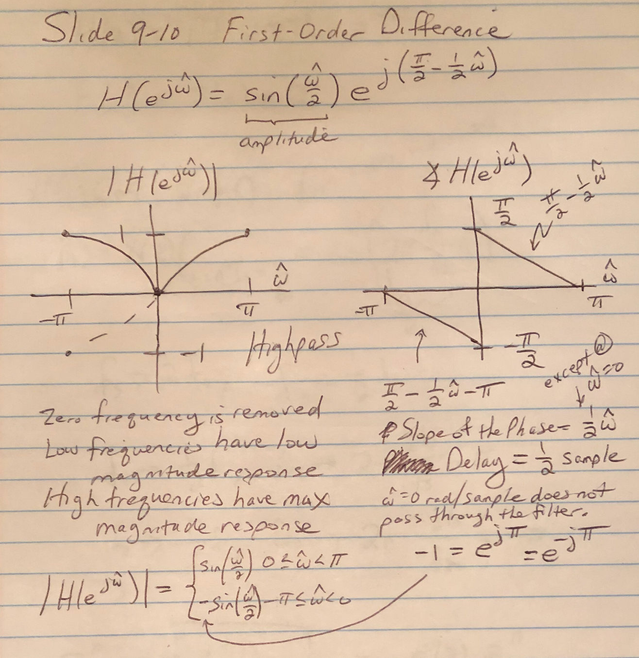
  Here are the visual effects after applying the first-order difference filter along each row or column of an image:

  • In the spatial domain (image pixel domain), each output sample of the 1-D first-order difference filter will be the current input value minus the previous input value. So, along one row of the echart image, because the echart image only has values of 0 and 255, will be one of the following outcomes:
    • -255 due to 0 - 255 = -255 when a white pixel (255) is followed by black pixel (0)
    • 0 due to either 0 - 0 or 255 - 255 when a black pixel (0) is followed by a black pixel (0) or a white pixel is followed by a white pixel
    • 255 due to 255 - 0 when a black pixel (0) is followed by a white pixel (255)
    In this case, -255 would correspond to black and 255 to a white in the grayscale image. Use imshow(image, []) so the pixel values are displayed full scale and not clipped.
  • In the frequency domain, the first-order difference filter is a highpass filter. When applied in either direction in a grayscale image, the filter will enhance the places where high frequencies occur, e.g. a sudden change from black to white or white to black. For the output image, the visual effect will be to extract lines, edges, texture, and other high frequency components.

  Here is my code for Section 2.5:

  % The load command will define a Matlab matrix echart.
  load echar512.mat
  
  % Display the image. 
  hAxes = axes(figure); 
  hImage = imshow(echart, [], 'Parent', hAxes);
  title(hAxes, 'Original echart image');
  
  % Apply a first-order difference filter along the rows.
  % Display the resulting image.
  bdiffh = [1, -1];
  yy1 = conv2(echart, bdiffh);
  hAxes1 = axes(figure); 
  hImage1 = imshow(yy1, [], 'Parent', hAxes1);
  title(hAxes1, 'echart image filtered with [1 -1] along the rows');
  
  % Apply a first-order difference filter along the columns.
  % Display the resulting image.
  bdiffh = [1, -1];
  yy2 = conv2(echart, bdiffh');
  hAxes2 = axes(figure); 
  hImage2 = imshow(yy2, [], 'Parent', hAxes2);
  title(hAxes2, 'echart image filtered with [1 -1] along the columns');
  

• Section 3.2: Image Restoration
  The image restoration approach being used is equalization. That is, filter #2 should do its best to compensate for the frequency distortion in the filter #1. Filter #2 is an equalizer.

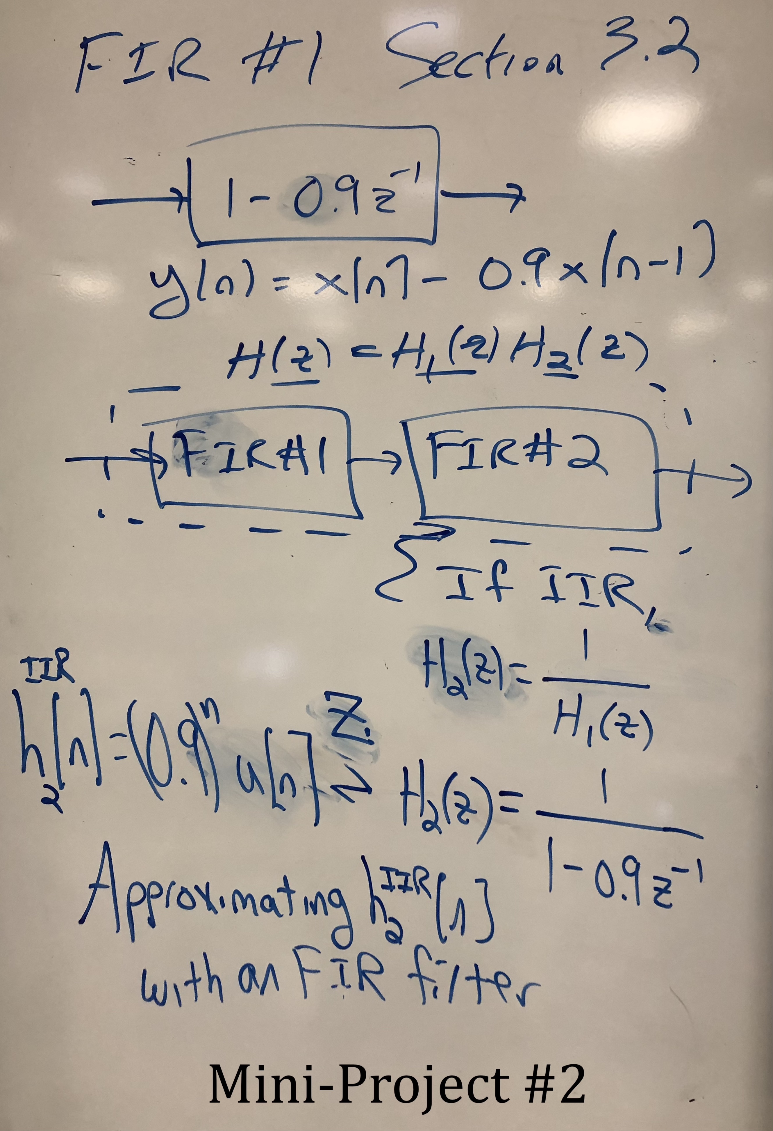
  Here is the Matlab code to define the 1-D impulse responses for 2-D LTI FIR filters 1 and 2:

  % h1[n] has non-zero coefficients of 1 and -q:
  q = 0.9;
  h1 = [ 1 -q ];
  
  % h2[n] = r^n for 0 <= n <= M and zero elsewhere:
  r = 0.9;
  M = 22;
  n = 0 : M;
  h2 = r .^ n;
  

  Here's the ideal image restoration filter and how it relates to the one we're using.

  Section 3.2.2 asks us to find the "worst case error in order to say how big the ghosts are relative to “black-white” transitions which are 0 to 255," and later in 3.3.3 we are asked to convert that error to a value in gray scale from 0 to 255. We can compute the worst case error on a pixel-by-pixel basis between image1 and image2 as follows where image1 and image2 would need to have the same dimensions:

  imageDiff = image1 - image2;
  imageDiffAbs = abs(imageDiff);
  imageDiffAbsWorstCase = max(max(imageDiffAbs));
  

  Note that max(ImageDiffAbs) takes the maximum of each row of imageDiffAbs. The mean squared error (MSE) would add the entries in imageDiffAbs, and the normalized mean square error would add the entries in imageDiffAbs and divide by the number of pixels.

  The lab asks you to find ways to compare two images. Matlab has several standard Image Quality Metrics:

  • immse to compute the mean squared error (MSE) where a lower score is better, but the scores might not align well with human perception of quality.
  • psnr to compute the peak signal-to-noise ratio (PSNR) in dB where a higher score is better, but the scores might not align well with human perception of quality.
  • ssim to compute the structural similarity (SSIM) index on a scale of 0 to 1 where a higher score is better, and the scores align well with human perception of quality.
  Please use all three. See the next item.

  Our reference image, echart, has 512 row and 512 columns. If you used the conv2 function, the images resulting from filtering echart are larger than echart, and we can crop the resulting image to be the same size as echart:

  ech90cropped = ech90(1:512, 1:512);
  

  We choose the first 512 columns in the first 512 rows because the convolution with the second filter will create large black borders on the right and on the bottom of the filtered image, and we'd like to remove the borders.

  You do not have to crop if you are using the filter function -- the filter function only outputs as many samples as are in the input signal.

Last updated 11/03/23. Send comments to bevans@ece.utexas.edu