Chapter 13: Digital to Analog Conversion and Sound
Modified to be compatible with EE319K Lab 6

Embedded Systems - Shape The World
Jonathan Valvano and Ramesh Yerraballi

 

As we have seen throughout this class, an embedded system uses its input/output devices to interact with the external world. Input devices allow the system to gather information about the world, and output devices can affect visual, mechanical, chemical, auditory, and biologic processes in the world. In this chapter we will literally “Shape The World”. We present a technique for the system to generate an analog output using a digital to analog converter (DAC). Together with periodic interrupts the system can generate waveforms, which are analog voltages that vary in time and in amplitude. We will then connect the waveform to a speaker and generate sound.

Learning Objectives: Develop a means for a digital computer to interact with the analog world. Study digitization: Quantization, range, precision and resolution. Introduce sampling and the Nyquist Theorem. Study the basics of sound: electromagnets, speakers, AC vs. DC power, perception of sound. Understand how to create sound: loudness, pitch, envelope, and shape Use SysTick to create sounds by programming variable frequencies.

Video 13.0. Introduction to Sound

	Sine wave 5 seconds of a 220 Hz sine wave
Problems playing this file? See media help.

 

An analog signal is one that is continuous in both amplitude and time. Neglecting quantum physics, most signals in the world exist as continuous functions of time in an analog fashion (e.g., voltage, current, position, angle, speed, force, pressure, temperature, and flow etc.) In other words, the signal has amplitude that can vary over time, but the value cannot instantaneously change. To represent a signal in the digital domain we must approximate it in two ways: amplitude quantizing and time quantizing (or Sampling). From an amplitude perspective, we will first place limits on the signal restricting it to exist between a minimum and maximum value (e.g., 0 to +3.3V), and second, we will divide this amplitude range into a finite set of discrete values. The range of the system is the maximum minus the minimum value. The precision of the system defines the number of values from which the amplitude of the digital signal is selected. Precision can be given in number of alternatives, binary bits, or decimal digits. The resolution is the smallest change in value that is significant. Furthermore, with respect to time one considers analog signals to exist from time equals minus infinity to plus infinity.  Because memory is finite, when representing signals on a digital computer, we will restrict signal to a finite time, or we could have a finite set of data that are repeated over and over.

Figure 13.1 shows a temperature waveform (solid line), with a corresponding digital representation sampled at 1 Hz and stored as a 5-bit integer number with a range of 0 to 31 ^oC. Because it is digitized in both amplitude and time, the digital samples (individual dots) in Figure 13.1 must exist at an intersection of grey lines. Because it is a time-varying signal (mathematically, this is called a function), we have one amplitude for each time, but it is possible for there to be 0, 1, or more times for each amplitude.

Figure 13.1. An analog signal is represented in the digital domain as discrete samples

Video 13.1. Fundamentals of Digitization

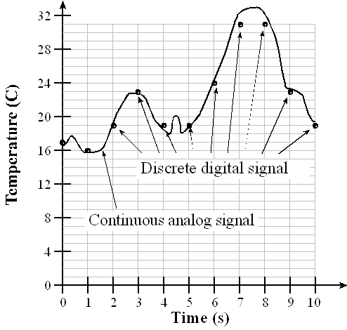
The second approximation occurs in the time domain. Time quantizing is caused by the finite sampling interval. For example, the data are sampled every 1 second in Figure 13.1. In practice we will use a periodic timer to trigger an analog to digital converter (ADC) to digitize information, converting from the analog to the digital domain. Similarly, if we are converting from the digital to the analog domain, we use the periodic timer to output new data to a digital to analog converter (DAC). The Nyquist Theorem states that if the signal is sampled with a frequency of f_s, then the digital samples only contain frequency components from 0 to ½ f_s. Conversely, if the analog signal does contain frequency components larger than ½ f_s, then there will be an aliasing error during the sampling process (performed with a frequency of f_s). Aliasing is when the digital signal appears to have a different frequency than the original analog signal. Also note, the digital data has 11 values at times 0 to 10, but no information before time=0, and no information after time=10.

 

Checkpoint 13.1: Why can’t the digital samples represent the little wiggles in the analog signal?

Checkpoint 13.2: Why can’t the digital samples represent temperatures above 31 ^oC?

Checkpoint 13.3: What range of frequencies is represented in the digital samples when the ADC is sampled once every millisecond?

Checkpoint 13.4: If I wanted to create an analog output wave with frequency components from 0 to 11 kHz, what is the slowest rate at which I could output to the DAC?

Proving the Nyquist Theorem mathematically is beyond the scope of this course, but we can present a couple examples to support the basic idea of the Nyquist Theorem: we must sample at a rate faster than twice the rate at which signal itself is oscillating.

                  

                     Video 13.2. The Nyquist Theorem Illustrated

Example 1) There is a long distance race with runners circling around an oval track and it is your job to count the number of times a particular runner circles the track. Assume the fastest time a runner can make a lap is 60 seconds. You want to read a book and occasionally look up to see where your runner is. How often to you have to look at your runner to guarantee you properly count the laps? If you look at a period faster than every 30 seconds you will see the runner at least twice per lap and properly count the laps. If you look at a period slower than every 30 seconds, you may only see the runner once per lap and not know if the runner is going very fast or very slow. In this case, the runner oscillates at most 1 lap per minute and thus you must observe the runner at a rate faster than twice per minute.

 

Example 2) You live on an island and want to take the boat back to the mainland as soon as possible. There is a boat that arrives at the island once a day, waits at the dock for 12 hours and then it sets sail to the mainland. Because of weather conditions, the exact time of arrival is unknown, but the boat will always wait at the dock for 12 hours before it leaves. How often do you need to walk down to the dock to see if the boat is there? If the boat is at the dock, you get on the boat and take the next trip back to the mainland. If you walk down to the dock every 13 hours, it is possible to miss the boat. However, if you walk down to the dock every 12 hours or less, you’ll never miss the boat. In this case, the boat frequency is once/day and you must sample it (go to the dock) two times/day. 

Interactive Tool 13.1

Discover the Nyquist Theorem. A Continuous waveform like Figure 13.1 is shown, V = 1.5 + 1*sin(2pi50t)+0.5*cos(2pi 200t). You may select the sampling rate and the precision (in bits) to see the signal captured. Notice that at sampling rates above 100 Hz you capture the essence of the 50Hz periodic wave, and above 400 Hz you capture the essence of both the 50 and 200 Hz waves. To “capture the essence” means the analog and digital signal go up and down at the same rate.

A DAC converts digital signals into analog form as illustrated in Figure 13.2. Although one can interface a DAC to a regular output port, most DACs are interfaced using high-speed synchronous protocols, like the SSI. For more information about SSI, see Embedded Systems: Real-Time Interfacing to ARM® Cortex™-M Microcontrollers, 2020, ISBN: 978-1463590154. The DAC output can be current or voltage. Additional analog processing may be required to filter, amplify, or modulate the signal. We can also use DACs to design variable gain or variable offset analog circuits.

The DAC precision is the number of distinguishable DAC outputs (e.g., 16 alternatives, 4 bits). The DAC range is the maximum and minimum DAC output (volts, amps). The DAC resolution is the smallest distinguishable change in output. The units of resolution are in volts or amps depending on whether the output is voltage or current. The resolution is the change in output that occurs when the digital input changes by 1. For most DACs there is a simple relationship between range precision and resolution.

                    Range(volts) = Precision(alternatives) • Resolution(volts)

Figure 13.2. A 4-bit DAC provides analog output.

Video 13.3. Design of a DAC circuit

Interactive Tool 13.2

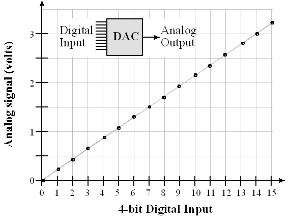
Learn about DAC precision using this tool. The analog output is fixed in the range 0 to 3.3V. You may adjust the number of bits from 1 to 10 to see how close the fit is to the straight line.

1 10 Number of DAC bits = 0

The DAC accuracy is (Actual - Ideal) / Ideal where Ideal is referred to the National Institute of Standards and Technology (NIST). One can choose the full scale range of the DAC to simplify the use of fixed-point math. For example, if an 8-bit DAC had a full scale range of 0 to 2.55 volts, then the resolution would be exactly 10 mV. This means that if the DAC digital input were 123, then the DAC output voltage would be 1.23 volts.

Checkpoint 13.5: A 10-bit DAC has a range of 0 to 2.5V, what is the approximate resolution?

Checkpoint 13.6: You need a DAC with a range of 0 to 2V, and a resolution of 1 mV. What is the smallest number of bits could you use for the DAC?

Example 13.1. Design a 2-bit binary-weighted DAC with a range of 0 to +3.3V using resistors.

Solution: We begin by specifying the desired input/output relationship of the 2-bit DAC. The design specifications are shown in Table 13.1.

 

N	Q1       Q0	Vout (V)
0	0    0	0.0
1	0    3.3	1.1
2	3.3  0	2.2
3	3.3  3.3	3.3

Table 13.1. Specifications of the 2-bit binary-weighted DAC.

 

Assume the output high voltage (V_OH) of the microcontroller is 3.3 V, and its output low voltage (V_OL) is 0. With a binary-weighted DAC, we choose the resistor ratio to be 2/1 so Q₁ bit is twice as significant as the Q₀ bit, as shown in Figure 13.3. Considering the circuit on the left (no headphones), if both Q₁ and Q₀ are 0, the output V_out is zero. If Q₁ is 0 and Q₀ is +3.3V, the output V_out is determined by the resistor divider network

 

                     

 

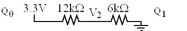
Note the total impedance from 3.3V to ground in the above circuit is 18kΩ. Using Ohm's Law, with the voltage divider equation, we can calculate V_out to be 3.3V*6kΩ/18kΩ, which is 1.1V. If Q₁ is +3.3V and Q₀ is 0, the output V_out is determined by the network

 

                   

 

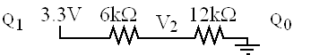
Again notice the total impedance from 3.3V to ground in this second circuit is 18kΩ. But this time we calculate V_out to be 3.3V*12kΩ/18kΩ, which is 2.2V. If both Q₁ and Q₀ are +3.3V, the output V_out is +3.3V. The output impedance of this DAC is approximately 12 kΩ, which means it cannot source or sink much current.

 

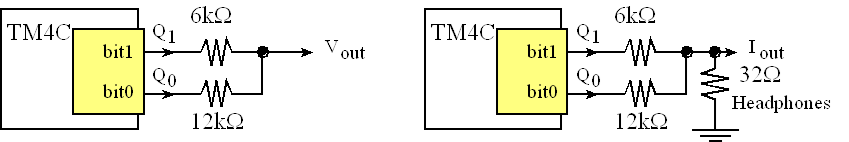
Figure 13.3. A 2-bit binary-weighted DAC.

If we connect headphones to this DAC, as shown in the right side of Figure 13.3, we could hear sounds generated by software writing a sequence of data to the DAC. However, since the impedance of the headphones is much smaller than the impedance of the DAC, the output voltages will be very small, but we could calculate the currents into the headphones. Considering the circuit on the right (with headphones), if both Q₁ and Q₀ are 0, the output current is zero. If Q₁ is 0 and Q₀ is +3.3V, the output current, I_out, is 3.3V divided by 12.032kΩ which is 0.275mA. If Q₀ is 0 and Q₁ is +3.3V, the output current, I_out, is 3.3V divided by 6.032kΩ which is 0.550mA. And finally, if both Q₁ and Q₀ are 3,3V, I_out is the sum of 0.275+0.550 (Kirkhoff's Current Law), which is about 0.825mA. Notice the current into the headphones is linearly related to the digital value. In other words, digital values of 0,1,2,3 map to currents of 0,0.275,0.550,0.825mA.

Interactive Tool 13.3

Shows how to compute Vout for the two scenarios bit1=0;bit0=1 and bit1=1;bit0=0. Using superposition, the scenario bit1=1;bit0=1 is simply the sum of the two cases: bit1=0;bit0=1 and bit1=1;bit0=0.

bit 0: 0V 3.3V bit 1: 0V 3.3V

You can realistically build a 6-bit DAC using the binary-weighted method.

Checkpoint 13.7: How do you build a 3-bit binary-weighted DAC using this method?

 

Before we generate sound, let’s look at how a typical speaker works. Sound exists as varying pressure waves that are created when a physical object moves, vibrating the air next to it. These air pressure waves travel through the air in all directions at about 343 m/sec. Sound can also be generated in water, where it travels at 1484 m/sec. Our ears can sense sounds from 20 Hz to about 20 kHz. In other words, the pressure wave must be oscillating faster than 20 Hz and slower than 20 kHz for us to hear it. See Figure 13.4.

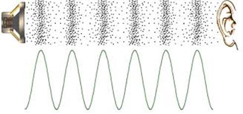
Figure 13.4. Sound waves exist as pressure waves in media such as air, water, and non-porous solids. For more information on sound, see http://www.mediacollege.com/audio/01/sound-waves.html

There are two magnets in a speaker. There is a large permanent magnetic that creates a static magnetic field oriented in the direction the speaker is facing, and there is a dynamic electromagnet created by a spiral-wound coil oriented in the same direction. Figure 13.5 shows a magnetic field generated by a cylindrically-wound coil.

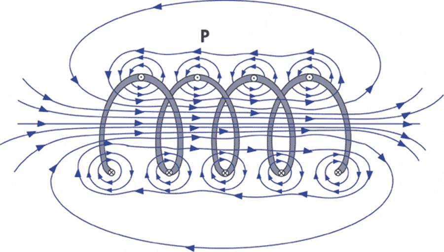
Figure 13.5. The magnetic field produced by a coil is very strong oriented in the direction of the cylinder. For more information on magnetic fields produced by a coil, see http://www.ndt-ed.org/EducationResources/CommunityCollege/MagParticle/Physics/CoilField.htm

The strength and direction of the magnetic field are related to the strength and direction of the electrical current conducted through the coiled wire. Figure 13.6 shows a cut away of a typical speaker. The alternating magnetic field generated by the coil interacts with the constant magnetic field produced by the permanent magnet. To generate sound we will create an oscillating current through the coil, this will create an oscillating magnetic field, and will vibrate the voice coil. The diaphragm and spider hold the voice coil to the suspension allowing it to vibrate up and down. When the voice coil vibrates up and down it creates sound waves. The frequency and amplitude of the sound is directly related to the frequency and amplitude of the current passing through the coil. The resistance of the coil in a typical headphone is 32 Ω.

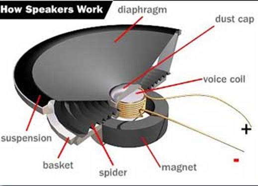
Figure 13.6. A speaker can generate sound by vibrating the voice coil using an electromagnet. For more information on speakers, see http://www.howstuffworks.com/speaker6.htm or http://www.audiocircuit.com/DIY/Dynamic-Speakers/Article:How-dynamic-loudspeakers-work

Checkpoint 13.8: Some speakers are heavier than others. These heavy speakers have larger permanent magnets. Why would we want a permanent magnet that can create a larger magnetic field?

                  

                     Video 13.6. how the speaker works

Most digital music devices rely on high-speed DACs to create the analog waveforms required to produce high-quality sound. In this section, we will discuss a very simple sound generation system that illustrates this application of the DAC. The hardware consists of a DAC and a speaker interface. You can drive headphones directly from a DAC output, but to drive a regular speaker, you will need to add an audio amplifier, as illustrated in Figure 13.7.

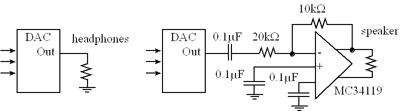
Figure 13.7. DAC allows the software to create music. For more information on the audio amplifier, refer to the data sheet of the MC34119. http://users.ece.utexas.edu/~valvano/Datasheets/MC34119.pdf

                  

                     Video 13.4. Sound as an analog signal: Loudness, pitch and shape

The quality of the music will depend on both hardware and software factors. The precision of the DAC, external noise, and the dynamic range of the speaker are some of the hardware factors. Software factors include the DAC output rate and the complexity of the stored sound data. If you output a sequence of numbers to the DAC that form a sine wave, then you will hear a continuous tone on the speaker, as shown in Figure 13.8. The loudness of the tone is determined by the amplitude of the wave. The pitch is defined as the frequency of the wave. Table 13.2 contains frequency values for the notes in one octave. The frequency of the wave, f_sin, will be determined by the frequency of the interrupt, f_int, divided by the size of the table n. The size of the table in Program 13.1 is n=16.

                                                            f_sin = f_int /n

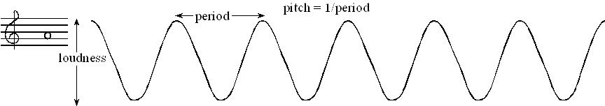
Figure 13.8. The loudness and pitch are controlled by the amplitude and frequency.

The frequency of each musical note can be calculated by multiplying the previous frequency by. You can use this method to determine the frequencies of additional notes above and below the ones in Table 13.2. There are twelve notes in an octave, therefore moving up one octave doubles the frequency.

Note	frequency
C	523 Hz
B	494 Hz
Bb	466 Hz
A	440 Hz
Ab	415 Hz
G	392 Hz
Gb	370 Hz
F	349 Hz
E	330 Hz
Eb	311 Hz
D	294 Hz
Db	277 Hz
C	262 Hz

Table 13.2. Fundamental frequencies of standard musical notes. The frequency for ‘A’ is exact.

 

 

Figure 13.9 illustrates the concept of instrument. You can define the type of sound by the shape of the voltage versus time waveform. Brass instruments have a very large first harmonic frequency.

 

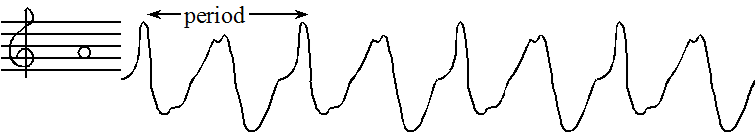
Figure 13.9. A waveform shape that generates a trumpet sound.

 

The tempo of the music defines the speed of the song. In 2/4 3/4 or 4/4 music, a beat is defined as a quarter note. A moderate tempo is 120 beats/min, which means a quarter note has a duration of ½ second. A sequence of notes can be separated by pauses (silences) so that each note is heard separately. The envelope of the note defines the amplitude versus time relationship. A very simple envelope is illustrated in Figure 13.10. The Cortex™-M processor has plenty of processing power to create these types of waves.

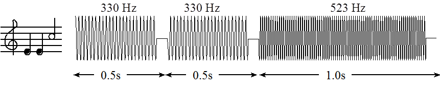
Figure 13.10. You can control the amplitude, frequency and duration of each note (not drawn to scale).

The smooth-shaped envelope, as illustrated in Figure 13.11, causes a less staccato and more melodic sound. This type of sound generation is possible to produce in real time on the Cortex™-M microcontroller.

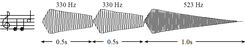
Figure 13.11. The amplitude of a plucked string drops exponentially in time.

A chord is created by playing multiple notes simultaneously. When two piano keys are struck simultaneously both notes are created, and the sounds are mixed arithmetically. You can create the same effect by adding two waves together in software, before sending the wave to the DAC. Figure 13.12 plots the mathematical addition of a 262 Hz (low C) and a 392 Hz sine wave (G), creating a simple chord.

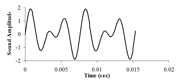
Figure 13.12. A simple chord mixing the notes C and G.

Example 13.2. Design a 3-bit R-2R DAC and use it to create a 100 Hz sine wave.

Video 13.5a. Design of a System that produces a 100Hz Sine Wave.

Video 13.5d. Construction of the DAC Circuit

Solution: We begin by specifying the desired input/output relationship of the 3-bit DAC. Table 13.3 shows the design specification. It will be able to generate 8 different current outputs with a resolution of about 12.5 μA. The circuit is presented in Figure 13.13.

 

N	Q2       Q1       Q0	Iout (μA)
0	0    0    0	0.0
1	0    0    3.3	12.5
2	0    3.3  0	25.0
3	0    3.3  3.3	37.5
4	3.3  0    0	50.0
5	3.3  0    3.3	62.5
6	3.3  3.3  0	75.0
7	3.3  3.3  3.3	87.5

Table 13.3. Specifications of the 3-bit R-2R DAC.

 

We assume the output high voltage (V_OH) of the microcontroller is 3.3 V, and its output low voltage (V_OL) is 0. A 3-bit R-2R DAC will use two R resistors (11kΩ) and five 2R resistors (22kΩ), as shown in Figure 13.13. The maximum current output will be (1/2 + 1/4 + 1/8)*3.3V/33kΩ = 87.5 μA.

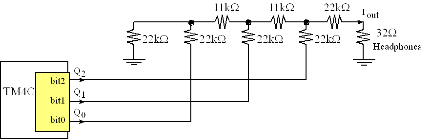
Figure 13.13. A 3-bit R-2R DAC.

 

The way to analyze an R-2R DAC is to employ the Law of Superposition. We will consider the three basis elements (1, 2, and 4). If these three cases are demonstrated, then the Law of Superposition guarantees the other five will work. When one of the digital inputs is true then V_ref (3.3V) is connected to the R-2R ladder, and when the digital input is false, then the connection is grounded. See Figure 13.14. Since 22,000 is much bigger than 32, we can neglect the 32-Ω resistance when calculating current.

Figure 13.14. Analysis of the three basis elements {001, 010, 100} of the 3-bit unsigned R-2R DAC.

Video 13.5b. Analysis of a R-2R Ladder circuit

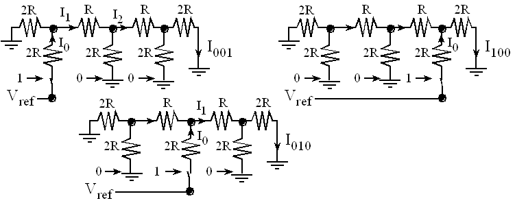
In each of the three test cases, the current across the active switch is I₀=V_ref / (3R). This current is divided by 2 at each branch point. I.e., I₁ = I₀/2, and I₂ = I₁/2. Current injected from the lower bits will be divided more times. Since each stage divides by two, the exponential behavior is produced. An actual DAC is implemented with a current switch rather than a voltage switch. Nevertheless, this simple circuit illustrates the operation of the R-2R ladder function. When the input is 001, V_ref is presented to the left. The effective impedance to ground is 3R, so the current injected into the R-2R ladder is I₀=V_ref / (3R). The current is divided in half three times, and I₀₀₁=V_ref / (24R).

When the input is 010, V_ref is presented in the middle. The effective impedance to ground is still 3R, so the current injected into the R-2R ladder is I₀=V_ref / (3R). The current is divided in half twice, and I₀₁₀=V_ref / (12R).

When the input is 100, V_ref is presented on the right. The effective impedance to ground is once again 3R, so the current injected into the R-2R ladder is I₀=V_ref / (3R). The current is divided in half once, and I₁₀₀=V_ref / (6R).

Using the Law of Superposition, the output voltage is a linear combination of the three digital inputs, I_out=(4b₂ + 2b₁ + b₀)V_ref / (24R). A current to voltage circuit is used to create a voltage output. To increase the precision one simply adds more stages to the R-2R ladder.

To generate sound we need a table of data and a periodic interrupt. Program 13.1 shows C code that defines a 16-element 3-bit sine wave. The frequency of the sound will be the interrupt frequency divided by 16 (size of the table). So, to create a 100 Hz wave we need SysTick to interrupt at 16*100 Hz, 1600 Hz. If the bus clock is 80 MHz, then the initialization should be called with an input parameter of value 50000. The const modifier will place the data in ROM.  The interrupt software will output one value to the DAC. See Figure 13.15. In this example, the 3-bit DAC is interfaced to output pins PB2-0. To output to this DAC we simply write to Port B. In order to create the sound, it is necessary to output just one number to the DAC upon each interrupt. The DAC range is 0 to 87.5 μA.

           

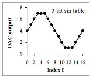
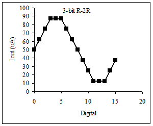
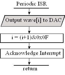
Figure 13.15. A DAC and a periodic interrupt are used to create sound. Output is discrete in time and voltage.

const uint8_t SineWave[16] = {4,5,6,7,7,7,6,5,4,3,2,1,1,1,2,3};

uint8_t Index=0;           // Index varies from 0 to 15

// **************DAC_Init*********************

// Initialize 3-bit DAC

// Input: none

// Output: none

void DAC_Init(void){uint32_t volatile delay;

  SYSCTL_RCGCGPIO_R |= 0x02; // activate port B

  delay = SYSCTL_RCGCGPIO_R;    // allow time to finish PortB clock activating

  GPIO_PORTB_DIR_R |= 0x07;      // make PB2-0 out

  GPIO_PORTB_DEN_R |= 0x07;      // enable digital I/O on PB2-0

}

 

// **************Sound_Init*********************

// Initialize Systick periodic interrupts

// Input: interrupt period

//        Units of period are 12.5ns

//        Maximum is 2^24-1

//        Minimum is determined by length of ISR

// Output: none

void Sound_Init(uint32_t period){

  DAC_Init();          // Port B is DAC

  Index = 0;

  NVIC_ST_CTRL_R = 0;         // disable SysTick during setup

  NVIC_ST_RELOAD_R = period-1;// reload value

  NVIC_ST_CURRENT_R = 0;      // any write to current clears it

  NVIC_SYS_PRI3_R = (NVIC_SYS_PRI3_R&0x00FFFFFF)|0x20000000; // priority 1

  NVIC_ST_CTRL_R = 0x0007; // enable SysTick with core clock and interrupts

}

// **************DAC_Out*********************

// output to DAC

// Input: 3-bit data, 0 to 7

// Output: none

void DAC_Out(uint32_t data){

  GPIO_PORTB_DATA_R = data;

}

// the sound frequency will be (interrupt frequency)/(size of the table)

void SysTick_Handler(void){

  Index = (Index+1)&0x0F;      // 4,5,6,7,7,7,6,5,4,3,2,1,1,1,2,3,... 

  DAC_Out(SineWave[Index]);    // output one value each interrupt

}

void main(void){

  PLL_Init();          // bus clock at 80 MHz

  Switch_Init();       // Port F is onboard switches, LEDs, profiling

  Sound_Init(50000);   // initialize SysTick timer, 1.6kHz

  while(1){

  }

}

Program 13.1. The periodic interrupt outputs one value to the DAC.

Video 13.5c. Program walkthrough

Video 13.5e. Demonstration of the Solution using a Scope

EE319K Lab 6 videos

Lab6_Introduction

In this video we review the software starter project and overview the design steps for implementing Lab 6.

                  

• Read: Book Chapter 6, eBook Chapters 12, 13
• Read: Lab 6 assignment
• Review: Lab 6 starter code
• Project structure, files, dac.xls
• Design/test: DAC_Init DAC_Out software
• Design/build/test: DAC circuit
• Design/test: Piano_Init Piano_In software
• Design/build/test: piano keyboard
• Design/test: Sound_Init, Sound_Play
• Design/test: main program

Lab6_Voltmeter

In this video we present the building and static testing of the DAC using a real voltmeter.

                  

This video used the following main program

int main(void){ // use this if you have a voltmeter
  TExaS_Init(SW_PIN_PE3210,DAC_PIN_PB3210,ScopeOn);  // bus clock at 80 MHz
  DAC_Init(); // your lab 6 solution
  Testdata = 15;
  EnableInterrupts();
  while(1){
    Testdata = (Testdata+1)&0x0F;
    DAC_Out(Testdata);  // your lab 6 solution
  }
}

Program 13.2. Main program for static testing if you have a voltmeter.

Lab6_Static

Building and static testing of the DAC using TExasDisplay as a voltmeter

                  

This video used the following main program

int main(void){ // use this if you do NOT have a voltmeter
uint32_t last,now;
  TExaS_Init(SW_PIN_PE3210,DAC_PIN_PB3210,ScopeOn); // bus clock at 80 MHz
  LaunchPad_Init(); // Initialized switches on PF0,PF4
  DAC_Init(); // your lab 6 solution
  Testdata = 15;
  EnableInterrupts();
  last = Switch_In();// read switches on PF0,PF4 (0x01 means PF0 touched)
  while(1){
    now = Switch_In();// 0 if no switch touched
    if((last != now)&&now){
      Testdata = (Testdata+1)&0x0F;
      DAC_Out(Testdata); // your lab 6 solution
    }
    last = now;
    Delay1ms(25); // debounces switch
  }
}

Program 13.3. Main program for static testing if you do NOT have a voltmeter.

Lab6_Dynamic

In this video we present the making of sound and dynamic testing of the DAC, using TExaSdisplay as a scope. The video includes a demonstration of a complete Lab 6 solution, including extra credit part.

                  

Lab6_Extra Credit

Extra credit Option 1 required you to create a data structure to hold music, convert sheet music to a sequence of notes, and to deploy a second periodic interrupt to manage the notes.

                  

There are two options for extra credit. This video outlines the approach to complete option 1. You can only complete only one of the options.

Lab6_Grading

Valvano pretends to be a student, Yerraballi pretends to be a TA, we show Valvano's screen and include Yerraballi's voice to demonstrate how the lab checkout will flow. For more flexibility you can connect to zoom with both your computer (to show deliverables, Keil, and TExaSdisplay) and your phone. You may find it easier to show your circuit with video from the phone.

                  

Reprinted with approval from Embedded Systems: Introduction to ARM Cortex-M Microcontrollers, 2020, ISBN: 978-1477508992, http://users.ece.utexas.edu/~valvano/arm/outline1.htm

and from Embedded Systems: Real-Time Interfacing to ARM® Cortex™-M Microcontrollers, 2020, ISBN: 978-1463590154, http://users.ece.utexas.edu/~valvano/arm/outline.htm