Appendix M. Math
Table of Contents:
- M.1. Interpolation
- M.2. Regression
- M.3. Cross Correlation
- M.4. Discrete Calculus
- M.5. Discrete Fourier Transform
- M.6. Digital Filter Design
- M.6.1. Basic Principles of Digital Signal Processing
- M.6.2. Multiple Access Circular Queue
- M.6.3. Using the Z-Transform to Derive Filter Response
- M.6.4. IIR Filter Design Using the Pole-Zero Plot
- M.6.5. FIR Filter Design
- M.7. Student's t-test
M.1. Interpolation
When a transducer is not linear, you could use a piece-wise linear interpolation to convert the ADC sample to temperature (D of 0.01 °C.) For more information on the circuit and its calibration, see Section 10.1 Measurement of Temperature. Figure M.1.1 shows a thermistor calibration curve with a nonlinear response. Program M.1.1 an example of a piece-wise linear interpolation There are two small tables Adata and Tdata. The Adata contains the ADC measurement results and the Tdata contains the corresponding temperature. The Adata table must be monotonic increasing. The ADC sample is passed into the lookup function. This function first searches the Adata for two adjacent points that surround the current ADC sample. Next, the function performs a linear interpolation to find the position that corresponds to the period sample. There are actually only 51 data points in the calibration tables, and points were added to the beginning and the end to handle possible temperatures over 40 or under 0 °C. Whenever subtraction occurs, it is best to use signed integer formats.
int32_t const Adata[53]={0,162,203,246,290,335,381,429,477,527,578,
630,684,738,795,852,911,971,1033,1096,1161,
1228,1296,1365,1437,1510,1584,1661,1739,1819,1901,
1985,2070,2158,2247,2338,2432,2527,2625,2724,2826,
2929,3035,3143,3253,3365,3479,3596,3714,3835,3958,4083,4096
};
int32_t const Tdata[53]={4000,4000,3920,3840,3760,3680,3600,3520,3440,3360,3280,
3200,3120,3040,2960,2880,2800,2720,2640,2560,2480,
2400,2320,2240,2160,2080,2000,1920,1840,1760,1680,
1600,1520,1440,1360,1280,1200,1120,1040,960,880,
800,720,640,560,480,400,320,240,160,80,0,0
};
int32_t Convert(int32_t data){ // data is 0 to 4095
int i=0;
while(data > Adata[i+1]){
i++; //search for Adata[i] < data <= Adata[i+1]
}
return (Tdata[i]+((Tdata[i+1]-Tdata[i])*(data-Adata[i]))/(Adata[i+1]-Adata[i]);
}
Program M.1.1. Linear Interpolation
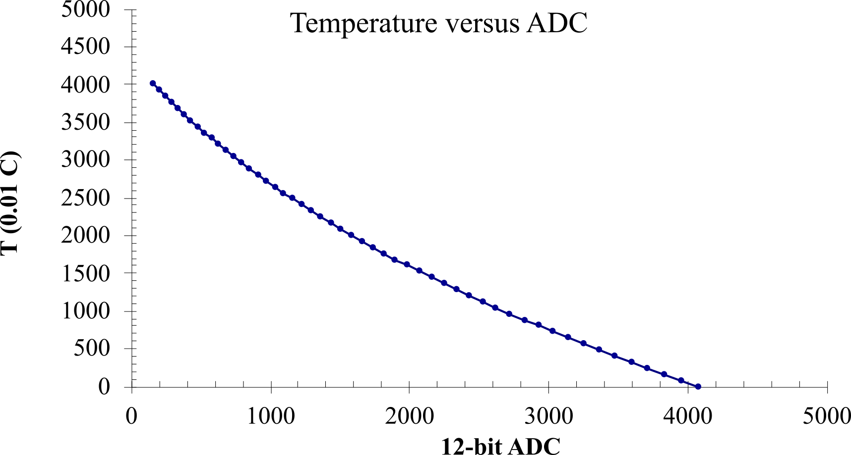
Figure M.1.1. Nonlinear sensor calibration curve.
In this example, we will design a fixed-point sin() function using table lookup and interpolation. The input is an 8-bit unsigned fixed-point with a resolution of 2p/256, and the output is an 8-bit signed fixed-point with a resolution of 1/127. Rather than have a complete table of all 256 possibilities, we will store a subset of individual points and use interpolation between the points, as shown in Table M.1.1 and Figure M.1.2. Let x be the input (0 ≤ x < 2p) and Ix be the integer portion (0 to 255). Similarly, y is the output (-1 ≤ y ≤ +1) and Iy is the integer portion (‑127 to 127). We need to create two unsigned 8-bit tables values containing the specific (input,output) pairs for the conversion. To make the table unsigned, we will store Iy+128 (offset binary).

Figure M.1.2. A table contains specific points, and the software will use linear interpolation to fill in the gaps.
The two lists consists of multiple unsigned (x,y) pairs, which define a piece-wise linear function. The first x entry must be less than or equal to minimum input, and the last x entry must be bigger than maximum input. The table must be monotonic increasing in x. See Program M.1.2. The test results of Program M.1.2 are plotted in Figure M.1.3.
|
index |
x |
y=sin(x) |
Ix |
Iy+128 |
|
0 |
0.000 |
0.000 |
0 |
128 |
|
1 |
0.314 |
0.309 |
13 |
167 |
|
2 |
0.628 |
0.588 |
26 |
203 |
|
3 |
0.942 |
0.809 |
38 |
231 |
|
4 |
1.257 |
0.951 |
51 |
249 |
|
5 |
1.571 |
1.000 |
64 |
255 |
|
6 |
1.885 |
0.951 |
77 |
249 |
|
7 |
2.199 |
0.809 |
90 |
231 |
|
8 |
2.513 |
0.588 |
102 |
203 |
|
9 |
2.827 |
0.309 |
115 |
167 |
|
10 |
3.142 |
0.000 |
128 |
128 |
|
11 |
3.456 |
-0.309 |
141 |
89 |
|
12 |
3.770 |
-0.588 |
154 |
53 |
|
13 |
4.084 |
-0.809 |
166 |
25 |
|
14 |
4.398 |
-0.951 |
179 |
7 |
|
15 |
4.712 |
-1.000 |
192 |
1 |
|
16 |
5.027 |
-0.951 |
205 |
7 |
|
17 |
5.341 |
-0.809 |
218 |
25 |
|
18 |
5.655 |
-0.588 |
230 |
53 |
|
19 |
5.969 |
-0.309 |
243 |
89 |
|
20 |
6.283 |
0.000 |
255 |
128 |
Table M.1.1. Fixed-point implementation of a sin function.
int32_t const IxTab[] = {0,13,26,38,51,64,77,90,102,115,128,141,
154,166,179,192,205,218,230,243,255};
int32_t const IyTab[] = {128,167,203,231,249,255,249,231,203,167,
128,89,53,25,7,1,7,25,53,89,128};
int32_t Convert(int32_t data){ // data is 0 to 4095
int i=0;
while(data > IxTab[i+1]){
i++; //search for IxTab[i] < data <= IxTab[i+1]
}
return (IyTab[i]+((IyTab[i+1]- IyTab[i])*(data- IxTab[i]))/( IxTab[i+1]- IxTab[i]);
}
Program M.1.2. Interpolation.
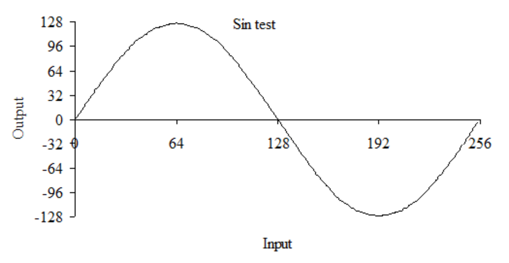

Figure M.1.3. Test results of Program M.1.2.
If speed is desired one could replace the small table with a complete table and just look up the answer. Program M.1.3 implements two sine and cosine functions without interpolation.
// index is angle in 0.001 radians
// index goes from 0 to 1571 (pi/2)
int16_t const SinTab[1572]={
0, 10, 20, 30, 40, 50, 60, 70, 80, 90, 100, 110, 120, 130, 140, 150, 160, 170, 180, 190, 200, 210, 220, 230, 240, 250, 260, 270,
280, 290, 300, 310, 320, 330, 340, 350, 360, 370, 380, 390, 400, 410, 420, 430, 440, 450, 460, 470, 480, 490, 500, 510, 520, 530,
540, 550, 560, 570, 580, 590, 600, 610, 620, 630, 640, 650, 660, 669, 679, 689, 699, 709, 719, 729, 739, 749, 759, 769, 779, 789,
799, 809, 819, 829, 839, 849, 859, 869, 879, 889, 899, 909, 919, 929, 939, 949, 959, 968, 978, 988, 998, 1008, 1018, 1028, 1038,
1048, 1058, 1068, 1078, 1088, 1098, 1108, 1118, 1128, 1138, 1147, 1157, 1167, 1177, 1187, 1197, 1207, 1217, 1227, 1237, 1247, 1257,
1267, 1277, 1286, 1296, 1306, 1316, 1326, 1336, 1346, 1356, 1366, 1376, 1386, 1395, 1405, 1415, 1425, 1435, 1445, 1455, 1465, 1475,
1484, 1494, 1504, 1514, 1524, 1534, 1544, 1554, 1564, 1573, 1583, 1593, 1603, 1613, 1623, 1633, 1643, 1652, 1662, 1672, 1682, 1692,
1702, 1712, 1721, 1731, 1741, 1751, 1761, 1771, 1780, 1790, 1800, 1810, 1820, 1830, 1839, 1849, 1859, 1869, 1879, 1889, 1898, 1908,
1918, 1928, 1938, 1947, 1957, 1967, 1977, 1987, 1996, 2006, 2016, 2026, 2036, 2045, 2055, 2065, 2075, 2085, 2094, 2104, 2114, 2124,
2133, 2143, 2153, 2163, 2173, 2182, 2192, 2202, 2212, 2221, 2231, 2241, 2251, 2260, 2270, 2280, 2290, 2299, 2309, 2319, 2328, 2338,
2348, 2358, 2367, 2377, 2387, 2396, 2406, 2416, 2426, 2435, 2445, 2455, 2464, 2474, 2484, 2493, 2503, 2513, 2522, 2532, 2542, 2551,
2561, 2571, 2580, 2590, 2600, 2609, 2619, 2629, 2638, 2648, 2658, 2667, 2677, 2687, 2696, 2706, 2715, 2725, 2735, 2744, 2754, 2764,
2773, 2783, 2792, 2802, 2812, 2821, 2831, 2840, 2850, 2860, 2869, 2879, 2888, 2898, 2907, 2917, 2927, 2936, 2946, 2955, 2965, 2974,
2984, 2993, 3003, 3012, 3022, 3032, 3041, 3051, 3060, 3070, 3079, 3089, 3098, 3108, 3117, 3127, 3136, 3146, 3155, 3165, 3174, 3184,
3193, 3203, 3212, 3222, 3231, 3240, 3250, 3259, 3269, 3278, 3288, 3297, 3307, 3316, 3325, 3335, 3344, 3354, 3363, 3373, 3382, 3391,
3401, 3410, 3420, 3429, 3438, 3448, 3457, 3467, 3476, 3485, 3495, 3504, 3513, 3523, 3532, 3541, 3551, 3560, 3569, 3579, 3588, 3598,
3607, 3616, 3625, 3635, 3644, 3653, 3663, 3672, 3681, 3691, 3700, 3709, 3718, 3728, 3737, 3746, 3756, 3765, 3774, 3783, 3793, 3802,
3811, 3820, 3830, 3839, 3848, 3857, 3867, 3876, 3885, 3894, 3903, 3913, 3922, 3931, 3940, 3949, 3959, 3968, 3977, 3986, 3995, 4004,
4014, 4023, 4032, 4041, 4050, 4059, 4068, 4078, 4087, 4096, 4105, 4114, 4123, 4132, 4141, 4151, 4160, 4169, 4178, 4187, 4196, 4205,
4214, 4223, 4232, 4241, 4250, 4259, 4268, 4277, 4287, 4296, 4305, 4314, 4323, 4332, 4341, 4350, 4359, 4368, 4377, 4386, 4395, 4404,
4413, 4422, 4431, 4439, 4448, 4457, 4466, 4475, 4484, 4493, 4502, 4511, 4520, 4529, 4538, 4547, 4556, 4564, 4573, 4582, 4591, 4600,
4609, 4618, 4627, 4636, 4644, 4653, 4662, 4671, 4680, 4689, 4697, 4706, 4715, 4724, 4733, 4742, 4750, 4759, 4768, 4777, 4785, 4794,
4803, 4812, 4821, 4829, 4838, 4847, 4856, 4864, 4873, 4882, 4890, 4899, 4908, 4917, 4925, 4934, 4943, 4951, 4960, 4969, 4977, 4986,
4995, 5003, 5012, 5021, 5029, 5038, 5047, 5055, 5064, 5073, 5081, 5090, 5098, 5107, 5116, 5124, 5133, 5141, 5150, 5159, 5167, 5176,
5184, 5193, 5201, 5210, 5218, 5227, 5235, 5244, 5252, 5261, 5269, 5278, 5286, 5295, 5303, 5312, 5320, 5329, 5337, 5346, 5354, 5363,
5371, 5379, 5388, 5396, 5405, 5413, 5422, 5430, 5438, 5447, 5455, 5463, 5472, 5480, 5489, 5497, 5505, 5514, 5522, 5530, 5539, 5547,
5555, 5564, 5572, 5580, 5589, 5597, 5605, 5613, 5622, 5630, 5638, 5646, 5655, 5663, 5671, 5679, 5688, 5696, 5704, 5712, 5720, 5729,
5737, 5745, 5753, 5761, 5770, 5778, 5786, 5794, 5802, 5810, 5818, 5827, 5835, 5843, 5851, 5859, 5867, 5875, 5883, 5891, 5900, 5908,
5916, 5924, 5932, 5940, 5948, 5956, 5964, 5972, 5980, 5988, 5996, 6004, 6012, 6020, 6028, 6036, 6044, 6052, 6060, 6068, 6076, 6084,
6092, 6100, 6107, 6115, 6123, 6131, 6139, 6147, 6155, 6163, 6171, 6178, 6186, 6194, 6202, 6210, 6218, 6226, 6233, 6241, 6249, 6257,
6265, 6272, 6280, 6288, 6296, 6303, 6311, 6319, 6327, 6334, 6342, 6350, 6358, 6365, 6373, 6381, 6388, 6396, 6404, 6412, 6419, 6427,
6435, 6442, 6450, 6457, 6465, 6473, 6480, 6488, 6496, 6503, 6511, 6518, 6526, 6533, 6541, 6549, 6556, 6564, 6571, 6579, 6586, 6594,
6601, 6609, 6616, 6624, 6631, 6639, 6646, 6654, 6661, 6669, 6676, 6684, 6691, 6698, 6706, 6713, 6721, 6728, 6735, 6743, 6750, 6758,
6765, 6772, 6780, 6787, 6794, 6802, 6809, 6816, 6824, 6831, 6838, 6846, 6853, 6860, 6867, 6875, 6882, 6889, 6896, 6904, 6911, 6918,
6925, 6933, 6940, 6947, 6954, 6961, 6969, 6976, 6983, 6990, 6997, 7004, 7011, 7019, 7026, 7033, 7040, 7047, 7054, 7061, 7068, 7075,
7082, 7089, 7096, 7104, 7111, 7118, 7125, 7132, 7139, 7146, 7153, 7160, 7167, 7174, 7181, 7187, 7194, 7201, 7208, 7215, 7222, 7229,
7236, 7243, 7250, 7257, 7264, 7270, 7277, 7284, 7291, 7298, 7305, 7311, 7318, 7325, 7332, 7339, 7345, 7352, 7359, 7366, 7373, 7379,
7386, 7393, 7400, 7406, 7413, 7420, 7426, 7433, 7440, 7446, 7453, 7460, 7466, 7473, 7480, 7486, 7493, 7500, 7506, 7513, 7519, 7526,
7533, 7539, 7546, 7552, 7559, 7565, 7572, 7578, 7585, 7591, 7598, 7604, 7611, 7617, 7624, 7630, 7637, 7643, 7650, 7656, 7663, 7669,
7675, 7682, 7688, 7695, 7701, 7707, 7714, 7720, 7726, 7733, 7739, 7745, 7752, 7758, 7764, 7771, 7777, 7783, 7790, 7796, 7802, 7808,
7815, 7821, 7827, 7833, 7839, 7846, 7852, 7858, 7864, 7870, 7877, 7883, 7889, 7895, 7901, 7907, 7913, 7920, 7926, 7932, 7938, 7944,
7950, 7956, 7962, 7968, 7974, 7980, 7986, 7992, 7998, 8004, 8010, 8016, 8022, 8028, 8034, 8040, 8046, 8052, 8058, 8064, 8070, 8076,
8081, 8087, 8093, 8099, 8105, 8111, 8117, 8123, 8128, 8134, 8140, 8146, 8152, 8157, 8163, 8169, 8175, 8180, 8186, 8192, 8198, 8203,
8209, 8215, 8220, 8226, 8232, 8238, 8243, 8249, 8255, 8260, 8266, 8271, 8277, 8283, 8288, 8294, 8299, 8305, 8311, 8316, 8322, 8327,
8333, 8338, 8344, 8349, 8355, 8360, 8366, 8371, 8377, 8382, 8388, 8393, 8398, 8404, 8409, 8415, 8420, 8425, 8431, 8436, 8442, 8447,
8452, 8458, 8463, 8468, 8474, 8479, 8484, 8490, 8495, 8500, 8505, 8511, 8516, 8521, 8526, 8532, 8537, 8542, 8547, 8552, 8558, 8563,
8568, 8573, 8578, 8583, 8588, 8594, 8599, 8604, 8609, 8614, 8619, 8624, 8629, 8634, 8639, 8644, 8649, 8654, 8659, 8664, 8669, 8674,
8679, 8684, 8689, 8694, 8699, 8704, 8709, 8714, 8719, 8724, 8728, 8733, 8738, 8743, 8748, 8753, 8758, 8762, 8767, 8772, 8777, 8782,
8786, 8791, 8796, 8801, 8805, 8810, 8815, 8820, 8824, 8829, 8834, 8838, 8843, 8848, 8852, 8857, 8862, 8866, 8871, 8876, 8880, 8885,
8889, 8894, 8898, 8903, 8908, 8912, 8917, 8921, 8926, 8930, 8935, 8939, 8944, 8948, 8953, 8957, 8961, 8966, 8970, 8975, 8979, 8984,
8988, 8992, 8997, 9001, 9005, 9010, 9014, 9018, 9023, 9027, 9031, 9036, 9040, 9044, 9048, 9053, 9057, 9061, 9065, 9070, 9074, 9078,
9082, 9086, 9091, 9095, 9099, 9103, 9107, 9111, 9115, 9119, 9124, 9128, 9132, 9136, 9140, 9144, 9148, 9152, 9156, 9160, 9164, 9168,
9172, 9176, 9180, 9184, 9188, 9192, 9196, 9200, 9204, 9208, 9211, 9215, 9219, 9223, 9227, 9231, 9235, 9238, 9242, 9246, 9250, 9254,
9257, 9261, 9265, 9269, 9272, 9276, 9280, 9284, 9287, 9291, 9295, 9298, 9302, 9306, 9309, 9313, 9317, 9320, 9324, 9328, 9331, 9335,
9338, 9342, 9346, 9349, 9353, 9356, 9360, 9363, 9367, 9370, 9374, 9377, 9381, 9384, 9388, 9391, 9394, 9398, 9401, 9405, 9408, 9411,
9415, 9418, 9422, 9425, 9428, 9432, 9435, 9438, 9441, 9445, 9448, 9451, 9455, 9458, 9461, 9464, 9468, 9471, 9474, 9477, 9480, 9484,
9487, 9490, 9493, 9496, 9499, 9502, 9505, 9509, 9512, 9515, 9518, 9521, 9524, 9527, 9530, 9533, 9536, 9539, 9542, 9545, 9548, 9551,
9554, 9557, 9560, 9563, 9566, 9569, 9572, 9574, 9577, 9580, 9583, 9586, 9589, 9592, 9594, 9597, 9600, 9603, 9606, 9608, 9611, 9614,
9617, 9619, 9622, 9625, 9628, 9630, 9633, 9636, 9638, 9641, 9644, 9646, 9649, 9651, 9654, 9657, 9659, 9662, 9664, 9667, 9670, 9672,
9675, 9677, 9680, 9682, 9685, 9687, 9690, 9692, 9695, 9697, 9699, 9702, 9704, 9707, 9709, 9711, 9714, 9716, 9719, 9721, 9723, 9726,
9728, 9730, 9733, 9735, 9737, 9739, 9742, 9744, 9746, 9748, 9751, 9753, 9755, 9757, 9759, 9762, 9764, 9766, 9768, 9770, 9772, 9774,
9777, 9779, 9781, 9783, 9785, 9787, 9789, 9791, 9793, 9795, 9797, 9799, 9801, 9803, 9805, 9807, 9809, 9811, 9813, 9815, 9817, 9819,
9820, 9822, 9824, 9826, 9828, 9830, 9832, 9833, 9835, 9837, 9839, 9841, 9842, 9844, 9846, 9848, 9849, 9851, 9853, 9854, 9856, 9858,
9860, 9861, 9863, 9865, 9866, 9868, 9869, 9871, 9873, 9874, 9876, 9877, 9879, 9880, 9882, 9883, 9885, 9887, 9888, 9890, 9891, 9892,
9894, 9895, 9897, 9898, 9900, 9901, 9902, 9904, 9905, 9907, 9908, 9909, 9911, 9912, 9913, 9915, 9916, 9917, 9918, 9920, 9921, 9922,
9923, 9925, 9926, 9927, 9928, 9930, 9931, 9932, 9933, 9934, 9935, 9936, 9938, 9939, 9940, 9941, 9942, 9943, 9944, 9945, 9946, 9947,
9948, 9949, 9950, 9951, 9952, 9953, 9954, 9955, 9956, 9957, 9958, 9959, 9960, 9961, 9961, 9962, 9963, 9964, 9965, 9966, 9967, 9967,
9968, 9969, 9970, 9971, 9971, 9972, 9973, 9974, 9974, 9975, 9976, 9976, 9977, 9978, 9978, 9979, 9980, 9980, 9981, 9982, 9982, 9983,
9983, 9984, 9984, 9985, 9986, 9986, 9987, 9987, 9988, 9988, 9989, 9989, 9990, 9990, 9990, 9991, 9991, 9992, 9992, 9992, 9993, 9993,
9994, 9994, 9994, 9995, 9995, 9995, 9996, 9996, 9996, 9996, 9997, 9997, 9997, 9997, 9998, 9998, 9998, 9998, 9998, 9999, 9999, 9999,
9999, 9999, 9999, 9999, 10000, 10000, 10000, 10000, 10000, 10000, 10000, 10000, 10000, 10000, 10000
};
//*********fixed-point sin****************
// input: -3142 to 3142, angle is in units radians/1000
// e.g., 90 degrees (pi/2 radians) is 1571
// output: -10000 to +10000, fixed point resolution 1/10000
int16_t fixed_sin(int32_t theta){
if(theta>3142) return 0;
if(theta<-3142) return 0;
if(theta<-1571) return -SinTab[3142+theta]; // -180 to -90 deg
if(theta<0) return -SinTab[-theta]; // -90 to 0 deg
if(theta<1571) return SinTab[theta]; // 0 to 90 deg
return SinTab[3142-theta]; // 90 to 180 deg
}
// cos(theta) = sin(pi/2-theta)
//*********fixed-point cos****************
// input: -3142 to 3142, angle is in units radians/1000
// e.g., 90 degrees (pi/2 radians) is 1571
// output: -10000 to +10000, fixed point resolution 1/10000
int16_t fixed_cos(int32_t theta){
if(theta>3142) return -10000;
if(theta<-3142) return -10000;
if(theta<-1571) return -SinTab[-1571-theta]; // -180 to -90 deg
if(theta<0) return SinTab[1571+theta]; // -90 to 0 deg
if(theta<1571) return SinTab[1571-theta]; // 0 to 90 deg
return -SinTab[-1571+theta]; // 90 to 180 deg
}
Program M.1.3. Fixed point trig functions
M.2. Regression
M.2.1. Linear Regression
Let xi be a set of inputs with yi being the corresponding output. If system is linear, then we can model the transfer function as a straight line, i.e., yi = mxi+b. We define the error of this linear equation as ei = (yi - mxi-b) for each point (xi,yi). The method of least squares finds m and b that minimizes, S, which is the sum of the squared error.
![]()
The least squares fit to yi = mxi+b can be derived by setting the two partial derivatives equal to zero (∂S/∂m=0 and ∂S/∂b = 0)

and

M.2.2. Nonlinear Regression
Considering the same (xi,yi) data points, we can still perform a regression (curve fit) even if the system is not linear. In general, we try to fit the data to the equation yi = f(xi) for some function f(x). For each data point, we define the error of this curve fit as ei = (yi - f(xi)). The function, f(x), will have one or more constant coefficients. For example, the step response of a linear system with one pole is
![]()
where ti are measured times and vi are measured outputs. This function is nonlinear having four constant coefficients: A0, A1, t0 and t. One way to perform the curve fit is to search the space of all values for the coefficients that minimizes mean squared error. I.e., find values of (A0, A1, t0 and t) that minimize
![]()
One approach to solving this problem is to reduce the number of coefficients. For example, if we can measure A0 and A1 independently, we can reduce the search space from 4 to 2 coefficients. The next step is to reformulate the problem into a linear function. It is still a nonlinear regression, but it is solved with linear regression tools. For this example, assuming A0 and A1 are known, we rewrite the function as
![]()
The function becomes linear with this mapping
![]()
When performing a nonlinear regression by reformulation, it is important to remember the process minimizes squared error on the linear variable. I.e., the previous example minimizes squared error between yi and mxi+b, and not the error between vi and A0+A1exp(-(ti-t0)/t).
Another example of a nonlinear curve fit involves calibration of a thermistor-based thermometer. A calibrated ohmmeter, a water bath and a calibrated thermometer are used to collect (Ri,Ti) data describing the thermistor response. The goal of the calibration is to be able to calculate temperature from measured resistance. The following empirical equation yields an accurate fit over a wide range of temperature:
![]()
where T is the temperature in °C, and R is the thermistor resistance in ohms. The cubic term was added to improve accuracy. It is preferable to use the ohmmeter function of the eventual instrument for calibration purposes so that influences of the resistance measurement hardware and software are incorporated into the calibration process.
The first step in the calibration process is to collect temperature (measured by a precision thermometer) and resistance data (measured by the ohmmeter process of the instrument). The thermistor(s) to be calibrated should be placed as close to the sensing element of the precision thermometer as possible. The water bath creates a stable yet controllable environment in which to perform the calibration. About 10 to 20 data points should be collected throughout the temperature range of interest.
The second step is to use nonlinear regression to determine H0, H1, and H3 from the collected data. The following nonlinear transforms will linearize the problem
x = lnR, y=(lnR)3, z= 1/(T+273.15)
where T is in °C. The problem is then transformed into the following linear equation
z = H0 + H1*x + H3*y
The linear regression finds (H0, H1, H3) that minimizes
![]()
The solution is found by setting the three partial derivatives equal to zero (∂S/∂H0=0 ∂S/∂H1=0 and ∂S/∂H3=0). Let n be the number of data points. Linear regression is used to determine the unknown coefficients from the x,y,z data. The following equations are used to calculate the coefficients H0,H1,H3 from the calibration data.
![]()
![]()
![]()
∆ = A11*A22 - (A12)2
![]()
![]()
![]()
![]()
![]()
M.3. Cross Correlation
There are many applications of cross correlation in the computer-based instrumentation field. We can use cross correlation to measure time delay (or phase shift) between two events, and we can use it to detect and classify events. The fundamental advantage of cross correlation over other methods like feature extraction is its insensitivity to noise. For continuous real variables, the cross correlation is defined as
![]()
where x(t) and y(t) are two infinite-time input waveforms. If the signal x(t) is the same shape as the signal y(t) delayed by t, the rxy(t) will be high. Figure M.3.1 shows a hardware implementation of the cross correlation.

Figure M.3.1. Hardware implementation of cross correlation
Inherent in the application of cross correlation in computer-based systems is the need to operate on finite sequences. Even virtual memory has a finite size, and most customers are not willing to wait for infinite time to get the results. The process of choosing a finite subsequence on which to operate is called windowing. It is critical to capture a reasonable window, because the data is considered as an infinite periodic signal. In other words, if we process the finite sequence
then the cross correlation will effectively be determined for the infinite sequence
..., x(0), x(1), x(2), ... x(N-1), x(0), x(1), x(2), ... x(N-1), x(0), x(1), x(2), ... x(N-1),...
Figures M.3.2 shows an improperly chosen window. Notice that the infinite periodic signal of Figure M.3.3 does not accurately represent the original data.
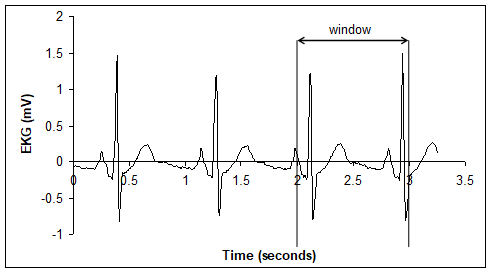
Figure M3.2. Original data with window from 2 to 3 seconds
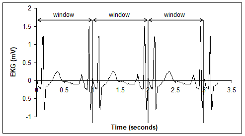
Figure M3.3. Equivalent infinite periodic signal resulting from the window shown in Figure M.3.2.
Figure M.3.4 shows a properly chosen window. Notice that the infinite periodic signal in Figure M.3.5 accurately represents the shape of the original data, but the information about heart rate is lost.
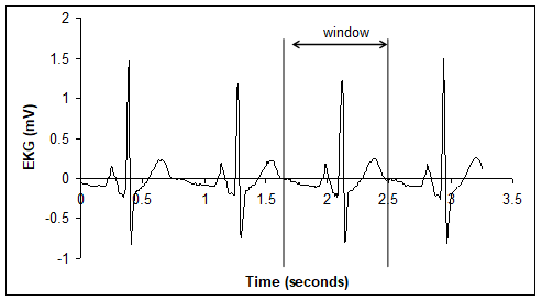
Figure M.3.4. Original data with window from 1.7 to 2.5 seconds
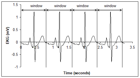
Figure M.3.5. Equivalent infinite periodic signal resulting from the window shown in Figure M.3.4.
If the window has multiple cycles, then there will be multiple correlations. To prevent multiple matches, we can choose a window with one cycle (like Figure M.3.4), or we can apply a mask to the data, as shown in Figure M.3.6. This is a trapezoidal mask, but other mask shapes can be used (rectangle, sine-wave, exponential). This method allows us to select a window without having to specify the sequence length. Notice that the window shown in Figure M.3.6 could be used to study the shape of just the QRS wave, without including the P and T waves.
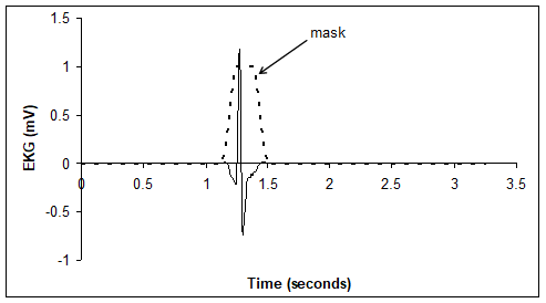
Figure M.3.6. A window is created by multiplying the original data with a mask.
To calculate the cross correlation on digitally-sampled data, we first calculate the average values. Assume x(n) and y(n) are the sampled data, and N is the sequence length. With bandpass systems such as EKG or sound, the averages may be zero.
![]()
![]()
The discrete cross covariance is a rough measure (not scaled to any particular value) of whether or not the signals x(n) and y(n) have the same shape. The delay parameter, equivalent to the t in the continuous case, is shown as m in the following definition of discrete cross covariance:
![]()
Notice that the discrete cross covariance is also a finite-length sequence, but it too can be considers as an infinite periodic sequence. The cross covariance of a signal with itself at delay equal to zero is similar to its variance
![]()
![]()
The discrete cross correlation between two finite sequences x(n) and y(n) is
![]()
The discrete autocorrelation can be calculated as the cross correlation of a signal and itself
![]()
In general, the cross correlation will be a number from -1 to +1. If rxy(m) equals 1 this means x(n) and y(n) time-shifted by m samples have exactly the same shape. If rxy(m) equals -1 this means x(n) and y(n) time-shifted by m samples have exactly the same shape, but inverted (upside down from each other). If rxy(m) equals 0 this means x(n) and y(n) time-shifted by m samples are not related to each other.
A typical application of cross correlation is event detection. Let y(n) contain a waveform that typifies the event for which we are searching. Let x(n) be real-time sampled data, windowed such that it has the same sequence length as y(n). Next we calculate rxy(m) for each value of m from 0 to N-1. If rxy(m) is above a threshold, we specify the event has occurred.
M.4. Discrete Calculus
Given a method to measure position, we can use calculus to determine velocity and acceleration.


The continuous derivative can be expressed as a limit.

The microcontroller can approximate the velocity be calculating the discrete derivative.

where ∆t is the time between velocity samples. At this point we introduce a short hand to describe digital samples. x(n) is the current sample, x(n-1) is the previous sample, and x(n-2) is the sample two times ago. When describing calculations performed on sampled data it is customary to use this notation. The use of n as the time variable emphasizes the signal exists only at discrete times.

This calculation of derivative is very sensitive to errors in the measurement of x(n). A more stable calculation averages two or more derivative terms taken over different time windows. In general we can define such a robust calculation as

If the integers p, m, and c are all positive, this calculation can be performed in real-time. The first term is the derivative over the large time window of p∆t. The second window term has a smaller size of m∆t. It normally fits entire inside the first with c>0 and c-m<p. The coefficients a and b create the weight for combining the short and long intervals. With a=b=1, p=3, m=1, and c=1, we get:

The acceleration can also be approximated by a discrete derivative.

Observation: In the above calculations of derivative, a single error in one of the x(t) input terms will propagate to only a finite number of the output calculations.
Observation: Although the central difference calculation of v(t)=(x(t+∆t)-x(t-∆t))/2∆t is theoretically valid, we cannot use it for real-time applications, because it requires knowledge about the future, x(t+∆t), which is unavailable at the time v(t) is being calculated.
Similarly, we can perform integration of velocity to determine position.

The microcontroller can perform discrete integration by summation.

There are two problems with this approach. The first difficulty is determining x(0). The second problem is the accumulation of errors. If one is calculating velocity from position and an error occurs in the measurement of x(n), then that error affects only two calculations of v(n). Unfortunately, if one is calculating position from velocity and an error occurs in the measurement of v(n), then that error will affect all subsequent calculations of x(n).
Observation: In the above calculation of integration, a single error in one of the x(t) input terms will propagate into all remaining output calculations.
The following function is a low pass digital filter.

Furthermore, if you sample an input at a regular rate, fs, then the following is a digital low pass filter with a cutoff of about fs /2k. This filter calculates the average of the last k samples.

: If you sample at 1000 Hz, how do you create a digital low pass filter with a cutoff of 10 Hz?
M.5. Discrete Fourier Transform
The Discrete Fourier Transform (DFT) converts data in the time domain to data in the frequency domain. We can use the DFT to measure SNR, to identify noise type, and to design FIR digital filters. In fact, the spectrum analyzer is simply a high-speed data acquisition system followed by a DFT. The Fast Fourier Transform (FFT) is a technique to calculate the DFT with fewer additions and multiplications. There are four important parameters when employing the DFT. The first parameter is sampling rate, fs. While the DFT deals only with samples and bins with no concept of volts, seconds, and Hz, when applying it to real data, we assume the samples have units, are bound by physical limits, and are evenly spaced at time intervals T=1/fs. The second parameter is sequence length, N. The other two parameters are input resolution and range. In real systems, input data comes from the ADC or input capture, and the output data go to the DAC or PWM. Therefore, the performance of the DFT will be affected by the range and resolution of the input. The input to the DFT will be N samples versus time, and the output will be N points in the frequency domain.
Input: {an} = {a0,a1,a2,...,aN-1}
Output: {Ak} = {A0,A1,A2,...,AN-1}
The definition of the DFT is
![]()
The DFT output Ak at index k represents the amplitude and phase of the input at frequency k*fS/N (in Hz). The DFT resolution in Hz/bin is the reciprocal of the total time spent gathering time samples; i.e., 1/(N*T). The Inverse Discrete Fourier Transform (IDFT) converts data in the frequency domain to data in the time domain. The input to the IDFT will be N points in the frequency domain, and the output will be N samples in the time domain.
Input: {Ak}={A0,A1,A2,...,AN-1}
Output: {an}={a0,a1,a2,...,aN-1}
The definition of the IDFT is
![]()
When presenting frequency data, we can use a log scale, making it easier to visualize frequency components with widely varying amplitudes. Because the system has physical limits, we use those limits to define full scale. Assume the audio system in Section 5.1.3 samples sound as a voltage from 0 to 3 V. For this system, we would define full scale VFS as 3 V. If V is a DFT output in volts, we can convert it to dB full scale using
dBFS = 20*log10(V/VFS)
STMicroelectronics published integer FFT code has part of their STM32F10x_DSP_Lib library. There are three separate FFT implementations for sizes 64, 256 or 1024 optimized for the Cortex M. The input to the FFT is 64, 256 or 1024 complex samples. Each input is a 16-bit signed integer containing the real and imaginary parts. For most applications we will set the ADC data into the real part, and we will write zeros into the imaginary part. In Program M.5.1 we fill the input array with constant data from an array. After calculating the DFT, the program will calculate the magnitude at each frequency. Let N be the size of the array, and assume the sampling rate is fs, then the meaning of index k is fs/N. The execution speed is shown in Table M.5.1.
typedef struct{
int16_t real,imag;
}Complex_t;
// data for FFT
Complex_t x[1024],y[1024]; // input and output arrays for FFT
int32_t mag[512]; // magnitude versus frequency of the output
void cr4_fft_1024_stm32(Complex_t *, Complex_t *, unsigned short);
int main(void){ int32_t t,k, real, imag;
for(t=0; t<1024; t=t+1){ // t means 1/fs
x[t].imag = 0; // imaginary part is zero
x[t].real = sinewave[t]; // fill real part with data
}
cr4_fft_1024_stm32(y, x, 1024); // complex FFT of 1024 values
for(k=0; k<512; k=k+1){ // k means fs/1024
real = y[k].real; // real is bottom 16 bits
imag = y[k].imag; // imag is top 16 bits
mag[k] = Sqrt(real*real+imag*imag);
}
while(1){};
}
Program M.5.1. Invoking the STM implementation of the FFT.
|
N |
Cycles |
Time(ms) |
|
64 |
3535 |
0.22 |
|
256 |
20072 |
1.25 |
|
1024 |
97870 |
6.12 |
Table M.5.1. Execution time of the FFT varies with N*log2(N).
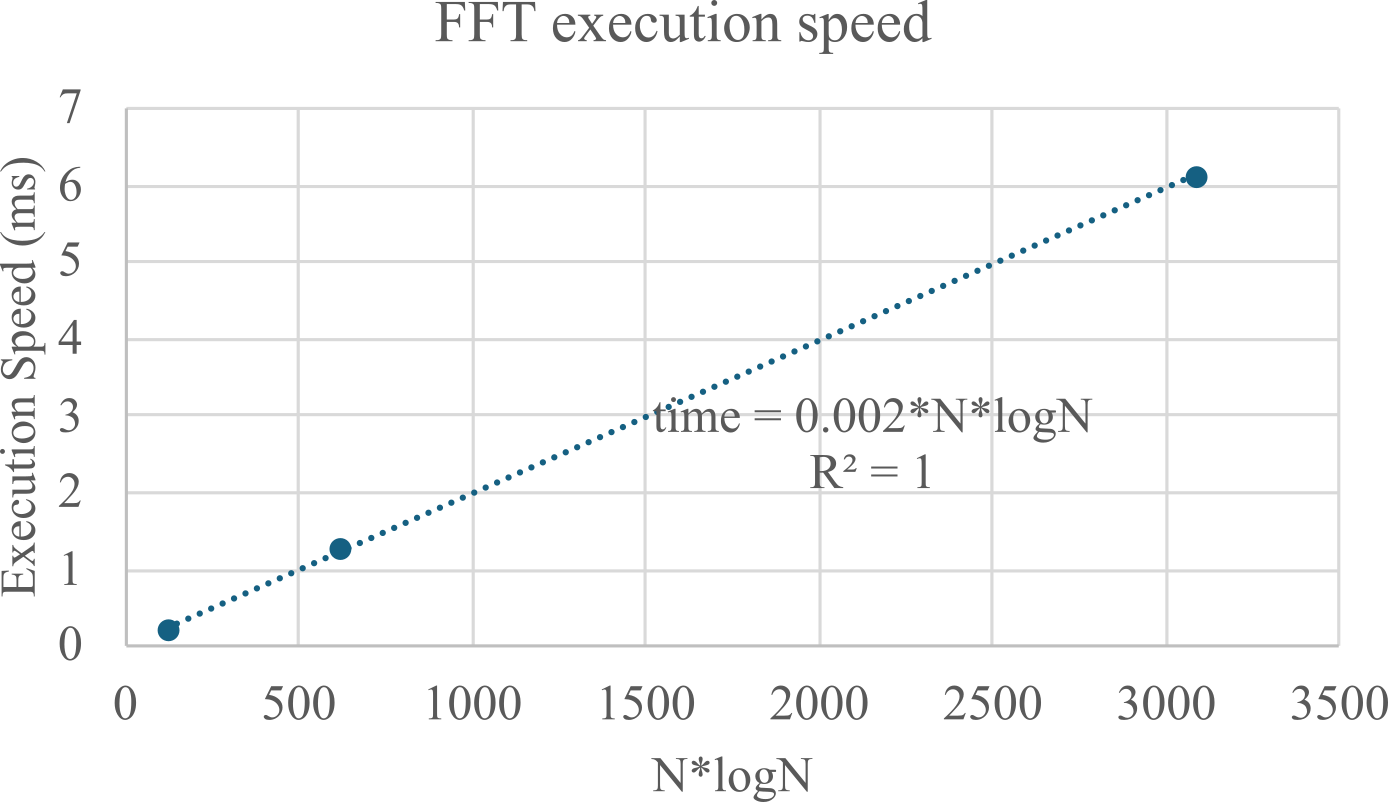
Figure M.5.1. Speed of FFT is N*logN
Program M.5.2 is a floating-point implementation of the FFT. It uses recursion to optimize execution speed. The complete code can be downloaded FFT.c and FFT.h. (**add links). The constants were generated with this fftdesign.xlsx spreadsheet. ***add link
/*
fft(v,N):
[0] If N==1 then return.
[1] For k = 0 to N/2-1, let ve[k] = v[2*k]
[2] Compute fft(ve, N/2);
[3] For k = 0 to N/2-1, let vo[k] = v[2*k+1]
[4] Compute fft(vo, N/2);
[5] For m = 0 to N/2-1, do [6] through [9]
[6] Let w.Real = cos(2*PI*m/N)
[7] Let w.Imag = -sin(2*PI*m/N)
[8] Let v[m] = ve[m] + w*vo[m]
[9] Let v[m+N/2] = ve[m] - w*vo[m]
Time to convert
n Time(us)
64 1659
128 3892
256 8979
512 20440
1024 46035
2048 102760
*/
void fft( complex_t *v, int n, complex_t *tmp ){
if(n>1) { /* otherwise, do nothing and return */
int k,m,j,n1;
complex_t z, w, *vo, *ve;
ve = tmp;
vo = tmp+n/2;
for(k=0; k<n/2; k++) {
ve[k] = v[2*k];
vo[k] = v[2*k+1];
}
fft( ve, n/2, v ); /* FFT on even-indexed elements of v[] */
fft( vo, n/2, v ); /* FFT on odd-indexed elements of v[] */
for(m=0; m<n/2; m++){
j = 0; n1 = 2;
while(n1<n){
j++; n1 = n1*2;
}
// j goes 0,1,2, 3, 4, 5, 6, 7, 8, 9, 10, 11
// n goes 2,4,8,16,32,64,128,256,512,1024,2048,4096
w.Real = cosTab[m][j];
w.Imag = -sinTab[m][j];;
// w.Real = cos(2*PI*m/(float)n);
// w.Imag = -sin(2*PI*m/(float)n);
z.Real = w.Real*vo[m].Real - w.Imag*vo[m].Imag; /* Re(w*vo[m]) */
z.Imag = w.Real*vo[m].Imag + w.Imag*vo[m].Real; /* Im(w*vo[m]) */
v[ m ].Real = ve[m].Real + z.Real;
v[ m ].Imag = ve[m].Imag + z.Imag;
v[m+n/2].Real = ve[m].Real - z.Real;
v[m+n/2].Imag = ve[m].Imag - z.Imag;
}
}
return;
}
/*
ifft(v,N):
[0] If N==1 then return.
[1] For k = 0 to N/2-1, let ve[k] = v[2*k]
[2] Compute ifft(ve, N/2);
[3] For k = 0 to N/2-1, let vo[k] = v[2*k+1]
[4] Compute ifft(vo, N/2);
[5] For m = 0 to N/2-1, do [6] through [9]
[6] Let w.Real = cos(2*PI*m/N)
[7] Let w.Imag = sin(2*PI*m/N)
[8] Let v[m] = ve[m] + w*vo[m]
[9] Let v[m+N/2] = ve[m] - w*vo[m]
*/
void ifft( complex_t *v, int n, complex_t *tmp ){
if(n>1) { /* otherwise, do nothing and return */
int k,m,j,n1;
complex_t z, w, *vo, *ve;
ve = tmp; vo = tmp+n/2;
for(k=0; k<n/2; k++){
ve[k] = v[2*k];
vo[k] = v[2*k+1];
}
ifft( ve, n/2, v ); /* FFT on even-indexed elements of v[] */
ifft( vo, n/2, v ); /* FFT on odd-indexed elements of v[] */
for(m=0; m<n/2; m++) {
j = 0; n1 = 2;
while(n1<n){
j++; n1 = n1*2;
}
// j goes 0,1,2, 3, 4, 5, 6, 7, 8, 9, 10, 11
// n goes 2,4,8,16,32,64,128,256,512,1024,2048,4096
w.Real = cosTab[m][j];
w.Imag = sinTab[m][j];;
// w.Real = cos(2*PI*m/(float)n);
// w.Imag = sin(2*PI*m/(float)n);
z.Real = w.Real*vo[m].Real - w.Imag*vo[m].Imag; /* Re(w*vo[m]) */
z.Imag = w.Real*vo[m].Imag + w.Imag*vo[m].Real; /* Im(w*vo[m]) */
v[ m ].Real = ve[m].Real + z.Real;
v[ m ].Imag = ve[m].Imag + z.Imag;
v[m+n/2].Real = ve[m].Real - z.Real;
v[m+n/2].Imag = ve[m].Imag - z.Imag;
}
}
return;
}
Program M.5.2. Floating point FFT
M.6. Digital Filter Design
M.6.1. Basic Principles of Digital Signal Processing
The objective of this section is to introduce simple digital filters. Let xc(t) be the continuous analog signal to be digitized. xc(t) is the analog input to the ADC converter. If fs is the sample rate, then the computer samples the ADC every T seconds. (T = 1/fs). Let . . . x(n),. . . be the ADC output sequence, where
x(n) = xc(nT) with -∞ < n < +∞.
There are two types of approximations associated with the sampling process. Because of the finite precision of the ADC, amplitude errors occur when the continuous signal, xc(t), is sampled to obtain the digital sequence, x(n). The second type of error occurs because of the finite sampling frequency. The Nyquist Theorem states that the digital sequence, x(n), properly represents the DC to ½fs frequency components of the original signal, xc(t). There are two important assumptions that are necessary to make when using digital signal processing:
1. We assume the signal has been sampled at a fixed and known rate, fs
2. We assume aliasing has not occurred.
We can guarantee the first assumption by using a hardware clock to start the ADC at a fixed and known rate. A less expensive but not as reliable method is to implement the sampling routine as a high priority periodic interrupt process. If the time jitter is δt then we can estimate the voltage error by multiplying the time jitter by the slew rate of the input, (∂V/∂t)*δt. By establishing a high priority of the interrupt handler, we can place an upper bound on the interrupt latency, guaranteeing that ADC sampling is occurring at an almost fixed and known rate. We can observe the ADC input with a spectrum analyzer to prove there are no significant signal components above ½fs. "No significant signal components" is defined as having an ADC input voltage |Z| less than the ADC resolution, ∆z,
|Z| ≤ ∆z for all f ≥ ½fs
A causal digital filter calculates y(n) from y(n-1), y(n-2),... and x(n), x(n-1), x(n‑2),... Simply put, a causal filter cannot have a nonzero output until it is given a nonzero input. The output of a causal filter, y(n), cannot depend on future data (e.g., y(n+1), x(n+1) etc.)
A linear filter is constructed from a linear equation. A nonlinear filter is constructed from a nonlinear equation. An example of a nonlinear filter is the median. To calculate the median of three numbers, one first sorts the numbers according to magnitude, then chooses the middle value. Other simple nonlinear filters include maximum, minimum, and square.
A finite impulse response filter (FIR) relates y(n) only in terms of x(n), x(n-1), x(n‑2),... If the sampling rate is 360 Hz, this simple FIR filter will remove 60 Hz noise:
y(n) = (x(n)+x(n-3))/2
An infinite impulse response filter (IIR) relates y(n) in terms of both x(n), x(n-1),..., and y(n‑1), y(n-2),... This simple IIR filter has averaging or low-pass behavior:
y(n) = (x(n)+y(n-1))/2
One way to analyze linear filters is the Z-Transform. The definition of the Z-Transform is:

The Z-transform is similar to other transforms. The Laplace Transform converts a continuous time-domain signal, x(t), into the frequency domain, X(s). In the same manner, the Z-Transform converts a discrete time sequence, x(n), into the frequency domain, X(z). See Figure M.6.1.

Figure M.6.1. A transform is used to study a signal in the frequency domain.
The input to both the Laplace and Z Transforms are infinite time signals, having values at times from -∞ to + ∞. The frequency parameters, s and z, are complex numbers, having real and imaginary parts. In both cases we apply the transform to study linear systems. We can describe the behavior (gain and phase) of an analog system using its transform, H(s) = Y(s)/X(s). In this same way we will use the H(z) transform of a digital filter to determine its gain and phase response. See Figure M.6.2.

Figure M.6.2. A transform can also be used to study a system in the frequency domain.
For an analog system we can calculate the gain by taking the magnitude of H(s) at s = j 2πf, for all frequencies, f, from -∞ to +∞. The phase will be the angle of H(s) at s = j 2πf. If we were to plot the H(s) in the s plane, the s = j 2πf curve is the entire y-axis. For a digital system we will calculate the gain and phase by taking the magnitude and angle of H(z). Because of the finite sampling interval, we will only be able to study frequencies from DC to ½fs in our digital systems. If we were to plot the H(z) in the z plane, the z curve representing the DC to ½fs frequencies will be the unit circle, z ≡ ej2πf/fs.
We will begin by developing a simple, yet powerful rule that will allow us to derive the H(z) transforms of most digital filters. Let m be an integer constant. We can use the definition of the Z-Transform to prove that:

For example, if X(z) is the Z-Transform of x(n), then z-3*X(z) is the Z-Transform of x(n-3). To find the Z-Transform of a digital filter, take the transform of both sides of the linear equation and solve for
![]()
To find the response of the filter, let z be a complex number on the unit circle
z = ej2πf/fs = cos(2πf/fs) + j sin(2πf/fs) for 0 ≤ f < ½fs
Let H(f) = a + bj, where a and b are real numbers. The gain of the filter is the complex magnitude of H(z) as f varies from 0 to ½fs.
![]()
The phase response of the filter is the angle of H(z) as f varies from 0 to ½fs.
![]()
Another way to analyze digital filters is to consider the filter response to particular input sequences. Two typical sequences are the step and the impulse (Figure M.6.3).
step ..., 0, 0, 0, 1, 1, 1, 1, ...
impulse ..., 0, 0, 0, 1, 0, 0, 0, ...
The impulse is defined as:
i(n) ≡ 1 for n = 0
0 for n ≠ 0
The step is defined as:
s(n) ≡ 0 for n < 0
1 for n ≥ 0
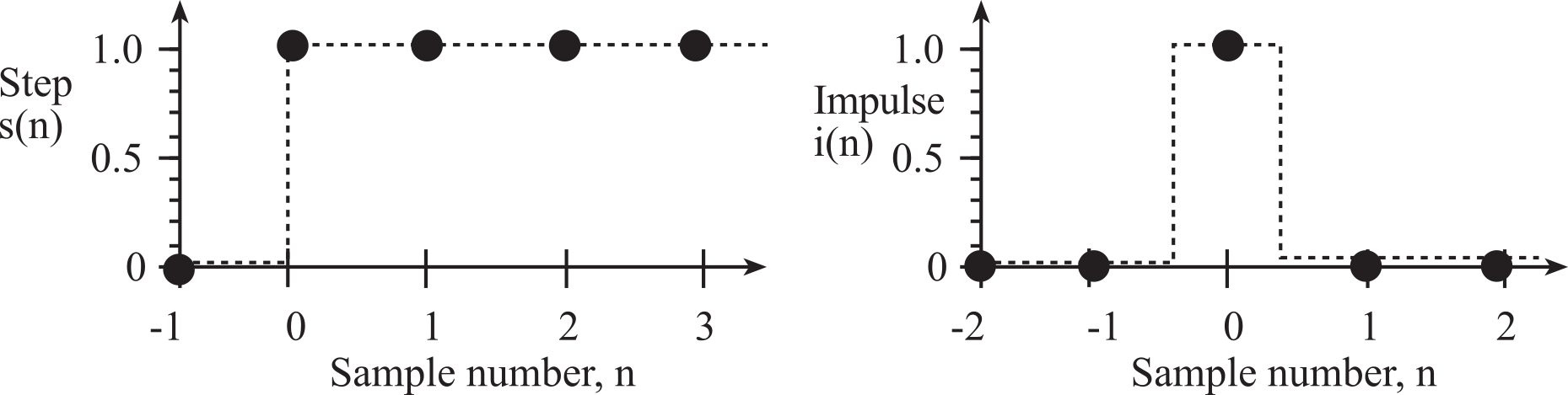
Figure M.6.3. Step and impulse inputs.
The step signal represents a sharp change (like an edge in a photograph). We will analyze three digital filters. The FIR is y(n) = (x(n)+x(n-1))/2. The IIR is y(n) = (x(n)+y(n-1))/2. The nonlinear filter is y(n) = median(x(n), x(n-1), x(n-2)). The median can be performed on any odd number of data points by sorting the data and selecting the middle value. The median filter can be performed recursively or nonrecursively. A nonrecursive 3-wide median filter is implemented in Program M.6.1.
uint8_t Median(uint8_t u1,uint8_t u2,uint8_t u3){
uint8_t result;
if(u1>u2){
if(u2>u3){
result = u2; // u1>u2,u2>u3 u1>u2>u3
}else{
if(u1>u3){
result = u3; // u1>u2,u3>u2,u1>u3 u1>u3>u2
}else{
result = u1; // u1>u2,u3>u2,u3>u1 u3>u1>u2
}
}
}else{
if(u3>u2){
result = u2; // u2>u1,u3>u2 u3>u2>u1
}else{
if(u1>u3){
result = u1; // u2>u1,u2>u3,u1>u3 u2>u1>u3
}else{
result = u3; // u2>u1,u2>u3,u3>u1 u2>u3>u1
}
}
}
return(result);
}
Program M.6.1: The median filter is an example of a nonlinear filter.
For a nonrecursive median filter, the original data points are not modified. For example, a 5-wide nonrecursive median filter takes as the filter output the median of {x(n), x(n-1), x(n-2), x(n-3), x(n-4)} On the other hand, a recursive median filter replaces the sample point with the filter output. For example, a 5-wide recursive median filter takes as the filter output the median of {x(n), y(n-1), y(n-2), y(n-3), y(n-4)} where y(n-1), y(n-2),... are the previous filter outputs. A median filter can be applied in systems that have impulse or speckle noise. Impulse or speckle noise causes one sample to be very different than the rest (like a speck on a piece of paper). The median filter will eliminate this type of noise. Except for the delay, the median filter passes a step without error. The step responses of the three filters are (Figure M.6.4):
FIR ..., 0, 0, 0, 0.5, 1, 1, 1, ...
IIR ..., 0, 0, 0, 0.5, 0.75, 0.88, 0.94, 0.97, 0.98, 0.99, ...
median ..., 0, 0, 0, 0, 1, 1, 1, 1, 1, ...
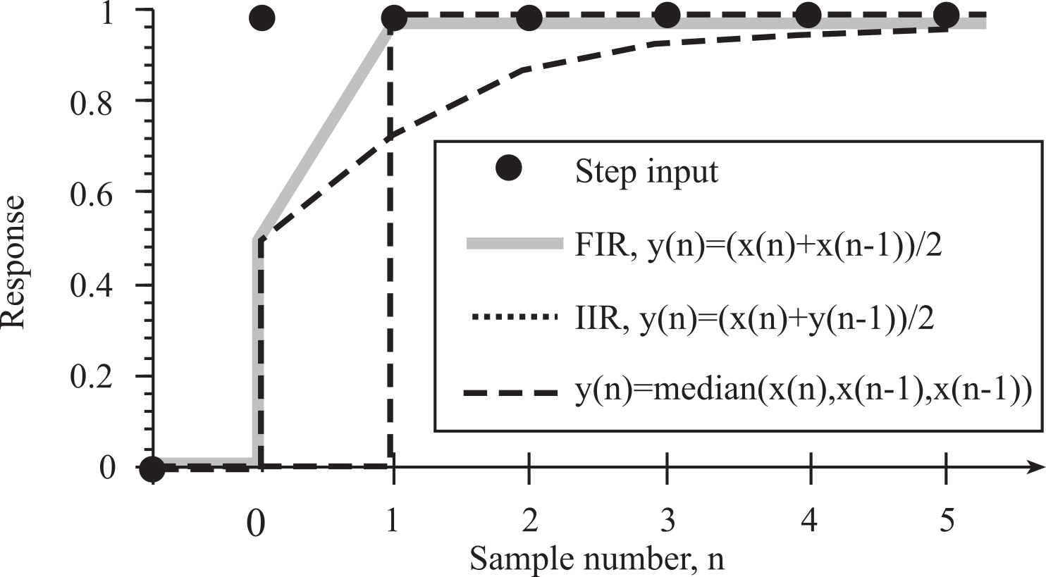
Figure M.6.4. Step response of three simple digital filters.
The impulse represents a noise spike (like spots on a Xerox copy). The impulse response of a filter is defined as h(n). The median filter completely removes the impulse. The impulse responses of the three filters are (Figure M.6.5):
FIR ..., 0, 0, 0, 0.5, 0.5, 0, 0, 0, ...
IIR ..., 0, 0, 0, 0.5, 0.25, 0.13, 0.06, 0.03, 0.02, 0.01, ...
median ..., 0, 0, 0, 0, 0, 0, 0, 0, ...
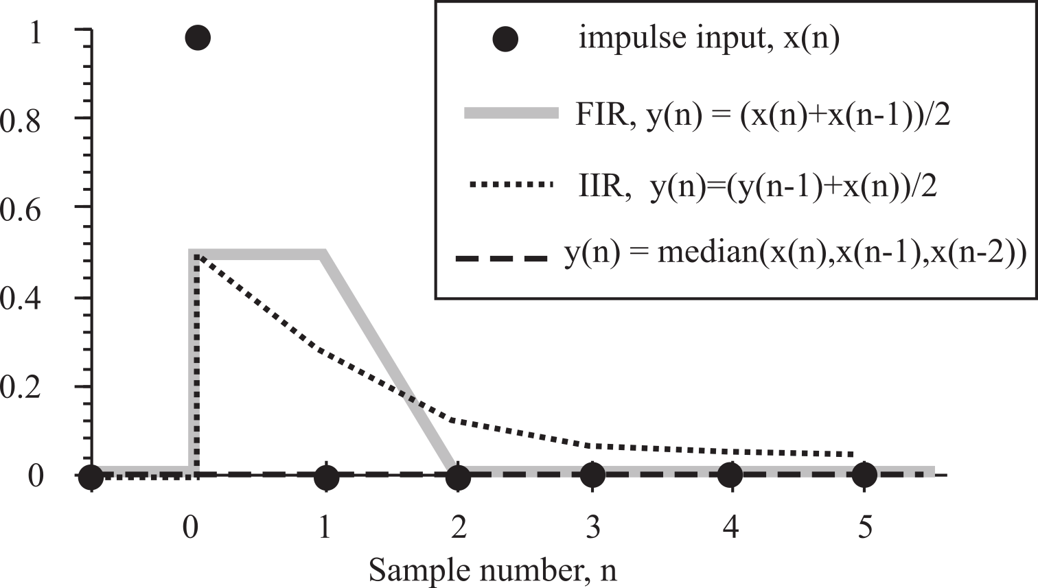
Figure M.6.5. Impulse response of three simple digital filters.
Note that the median filter preserves the sharp edges and removes the spike or impulsive noise. The median filter is nonlinear, and hence H(z) and h(n) are not defined for nonlinear filters. For linear filters, the impulse response, h(n), can also be used as an alternative to the transfer function H(z). h(n) is sometimes called the direct form. A causal filter has h(n) = 0 for n less than 0. For a casual filter.

For a finite impulse response (FIR) filter, h(n) = 0 for n ≥ N for some finite N. Thus,

The output of a filter can be calculated by convolving the input sequence, x(n), with h(n). For an infinite impulse response filter:

For a finite impulse response (FIR) filter:

M.6.2. Multiple Access Circular Queue
A multiple access circular queue (MACQ) is used for data acquisition and control systems. A MACQ is a fixed-length order-preserving data structure, containing the list N samples. When the MACQ hold just a few data points, it can be implemented like Figure M.6.6. When the MACQ holds many data points, it can be implemented using a pointer or index to the newest data, as presented in **Section 2.6.2***. The source process (ADC sampling software) places information into the MACQ. Once initialized, the MACQ is always full. The oldest data is discarded when the newest data is Put into a MACQ. The sink process can read any of the data from the MACQ. The Read function is non-destructive. This means that the MACQ is not changed by the Read operation. In this MACQ, the newest sample, x(n), is stored in element x[0]. x(n-1), is stored in element x[1].
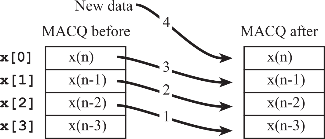
Figure M.6.6. When data is put into a multiple access circular queue, the oldest data is lost.
To Put data into this MACQ, four steps are followed, as shown in Figure M.6.6. First, the data is shifted down (steps 1, 2, 3), and then the new data is entered into the x[0] position (step 4).
The drawing in Figure M.6.6 shows the position in memory of x(n), x(n-1),... does not move when one data sample is added. Notice however, the data itself does move. As time passes the data gets older, the data moves down in the MACQ.
A simple application of the MACQ is the real-time calculation of derivative. Also assume the ADC sampling is triggered every 1 ms. x(n) will refer to the current sample, and x(n-1) will be the sample 1 ms ago. There are a couple of ways to implement a discrete time derivative. The simple approach is
![]()
In practice, this first order equation is quite susceptible to noise. An approach generating less noise calculates the derivative using a higher order equation like
![]()
The C implementation of this discrete derivative uses a MACQ (Program M.6.2). Since ∆t is 1 ms, we simply consider the derivative to have units mV/ms and not actually execute the divide by ∆t operation. Signed arithmetic is used because the slope may be negative.
int32_t x[4]; // MACQ (mV)
int32_t d; // derivative(V/s)
void SysTick_Handler(void){
x[3] = x[2]; // shift data
x[2] = x[1]; // units of mV
x[1] = x[0];
x[0] = (3000*ADC_In())>>12; // in mV
d = x[0]+3*x[1]-3*x[2]-x[3]; // in V/s
Fifo_Put(d); // pass to foreground
}
Program M.6.2. Software implementation of first derivative using a multiple access circular queue.
M.6.3. Using the Z-Transform to Derive Filter Response
In this section, we will use the Z-Transform to determine the digital filter response (gain and phase) given the filter equation. The first example is the average of the current sample with the sample 3 times ago. Program M.6.3 shows the implementation.
y(n) = (x(n)+x(n-3))/2
The first step is to take the Z-Transform of both sides of the equation. The Z-Transform of y(n) is Y(z), the Z-Transform of x(n) is X(z), and the Z-Transform of x(n-3) is z-3X(z). Since the Z-Transform is a linear operator, we can write:
Y(z) = (X(z) + z-3X(z))/2
The next step is to rewrite the equation in the form of H(z) ≡ Y(z)/X(z).
H(z) ≡ Y(z)/X(z) = ½ (1 + z-3)
We plug in z ≡ ej2πf/fs calculate the gain and phase response, see Figures M.6.7 and M.6.8.
H(f) = ½ (1 + e-j6πf/fs) = ½ (1 + cos(6πf/fs) - j sin(6πf/fs) )
Gain ≡ |H(f)| = ½ sqrt((1 + cos(6πf/fs))2 + sin(6πf/fs)2 ))
Phase ≡ angle(H(f)) = tan-1(-sin(6πf/fs)/(1 + cos(6πf/fs))
int32_t x[4]; // MACQ
void SysTick_Handler(void){ int32_t y;
x[3] = x[2]; // shift data
x[2] = x[1]; // units, ADC sample 0 to 4095
x[1] = x[0];
x[0] = ADC_In(); // 0 to 4095
y = (x[0]+x[3])/2; // filter output
Fifo_Put(y); // pass to foreground
}
Program M.6.3. If the sampling rate is 360 Hz, this filter rejects 60 Hz.
: If the sampling rate in Program M.6.3 is 360 Hz, use the Z transform to prove the 60 Hz gain is zero.
Observation: Program M.6.3 is double-notch filter rejecting ⅙ and ½ fs.
The second example is the average of the current sample with the previous filter output. Program M.6.4 shows the implementation
y(n) = (x(n)+y(n-1))/2
The first step is to take the Z-Transform of both sides of the equation. The Z-Transform of y(n) is Y(z), the Z-Transform of x(n) is X(z), and the Z-Transform of y(n-1) is z-1Y(z). Since the Z-Transform is a linear operator, we can write:
Y(z) = (X(z) + z-1Y(z))/2
The next step is to rewrite the equation in the form of H(z) ≡ Y(z)/X(z).
H(z) ≡ Y(z)/X(z) = 1/(2 - z-1)
We plug in z ≡ ej2πf/fs calculate the gain and phase response, see Figures M.6.7 and M.6.8.
H(f) = 1/(2 - e-j2πf/fs) = 1/(2 - cos(2πf/fs) + j sin(2πf/fs) )
Gain ≡ |H(f)|
Phase ≡ angle(H(f))
int32_t y;
void SysTick_Handler(void){ int32_t x;
x = ADC_In(); // 0 to 4095
y = (x+y)/2; // filter output
Fifo_Put(y); // pass to foreground
}
Program M.6.4. Implementation of an IIR low pass digital filter.
: For f between 0 and 0.2 fs, the filter in Program M.6.4 has a gain larger than 1 (see Figure M.6.7). What does that mean?
The gain of four linear digital filters is plotted in Figure M.6.7 and the phase response is plotted in Figure M.6.8.

Figure M.6.7. Gain versus frequency response for four simple digital filters.
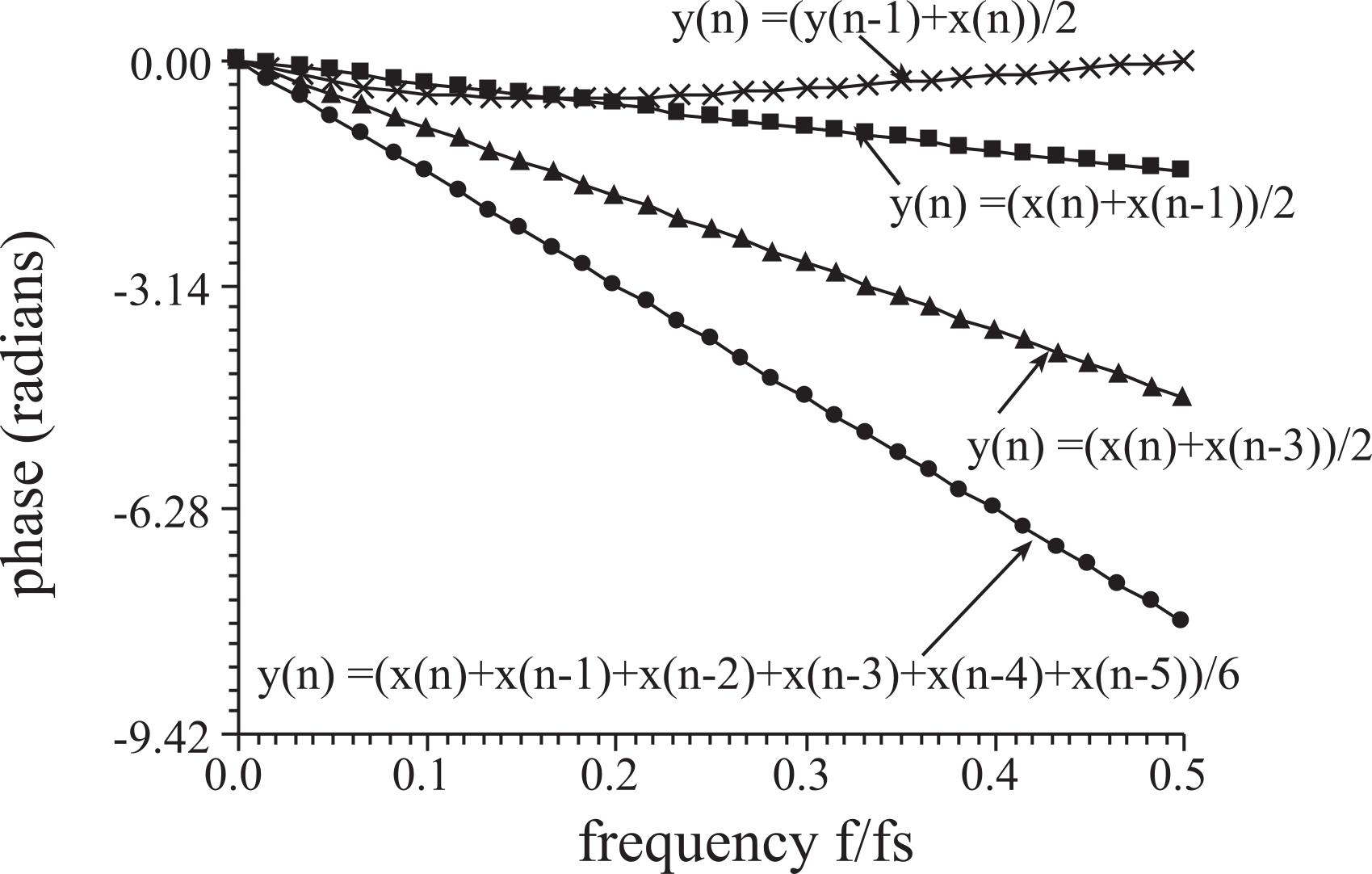
Figure M.6.8. Phase versus frequency response for four simple digital filters.
A linear phase versus frequency response is desirable because a linear phase causes minimal waveform distortion. Conversely, a nonlinear phase response will distort shape or morphology of the signal. In general, if fs is 2*k*fc Hz (where k is any integer k≥2), then the following is a fc notch filter:
![]()
Averaging the last k samples will perform a low-pass filter with notches. Let fc be the frequency we wish to reject. We will choose the sampling at a multiple of this notch. I.e., we choose fs to be k*fc Hz (where k is any integer k≥2), then the k-sample average filter will reject fc and its harmonics: 2fc, 3fc... If the number of terms k is large, the straight forward implementation of average will run slowly. Fortunately, this averaging filter can be rewritten as a function of the current sample x(n), the sample k times ago x(n-k), and the last filter output y(n-1).
![]()
The second formulation looks like an IIR filter, but it is a FIR filter because the equations are identical. The H(z) transfer function for this k-term averaging filter is
![]()
This class of digital low-pass filters can be implemented with a k+1 multiple access circular queue, and a simple calculation. The gain of this class of filter is shown in Figure M.6.9 for a sampling rate of 100 Hz.
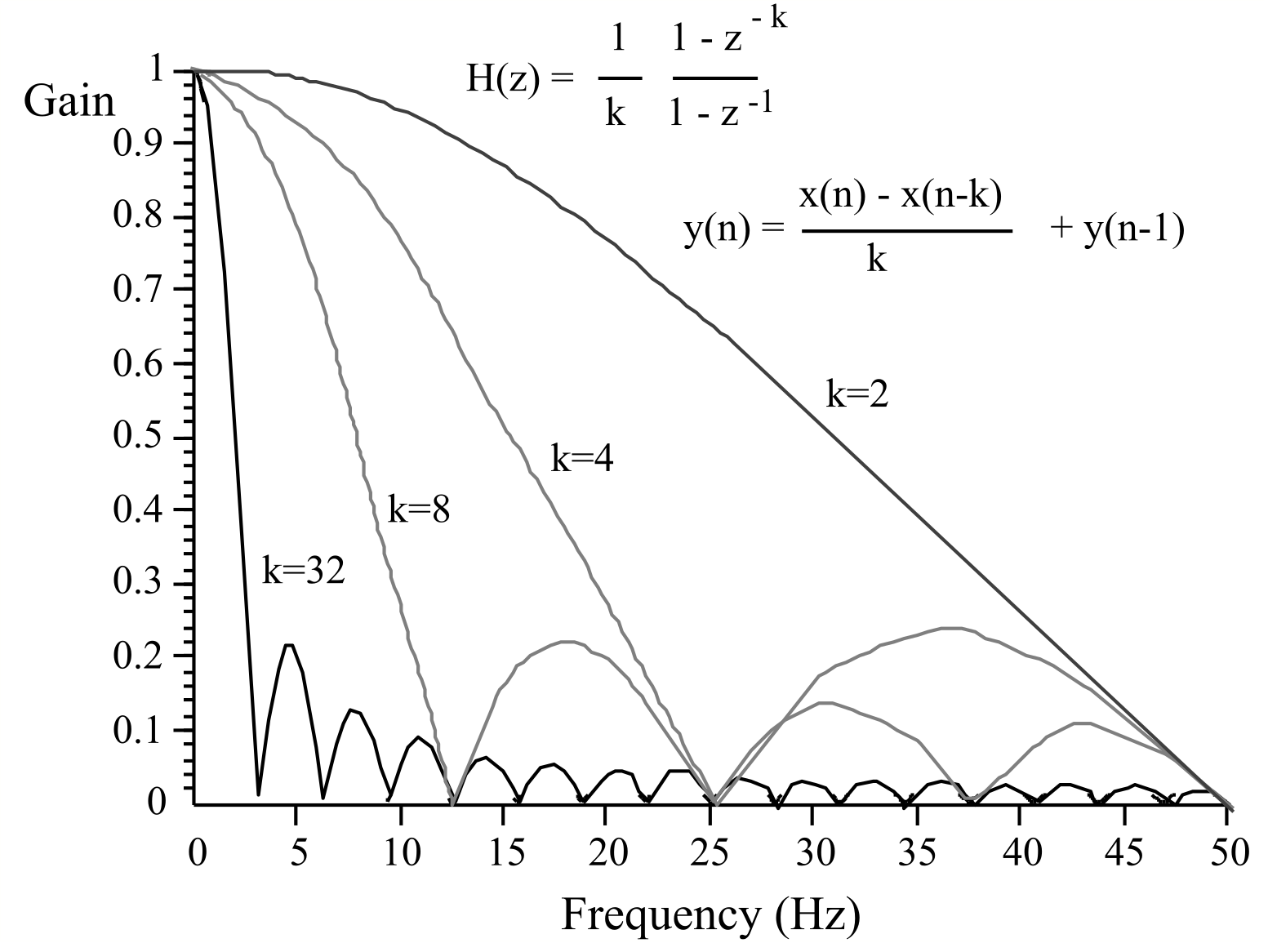
Figure M.6.9. Gain versus frequency plot of four averaging low-pass filters.
M.6.4. IIR Filter Design Using the Pole-Zero Plot
The objective of this section is to show the IIR filter design method using pole-zero plots. One starts with a basic shape in mind, and places poles and zeros to generate the desired filter. Consider again the analogy between the Laplace and Z Transforms. When the H(s) transform is plotted in the s plane, we look for peaks (places where the amplitude H(s) is high) and valleys (places where the amplitude is low.) We usually can identify zeros and poles. A zero is a place where H(s)=0. A pole is a place where H(s)=∞. In the same way, we can plot the H(z) in the z plane and identify the poles and zeros. Table M.6.1 lists the filter design strategies.
|
Analog condition |
Digital condition |
Consequence |
|
zero near s=j2πf line |
zero near z=ej2πf/fs |
low gain at the f near the zero |
|
pole near s=j2πf line |
pole near z=ej2πf/fs |
high gain at the f near the pole |
|
zeros in complex conjugate pairs |
zeros in complex conjugate pairs |
the output y(t) is real |
|
poles in complex conjugate pairs |
poles in complex conjugate pairs |
the output y(t) is real |
|
poles in left half plane |
poles inside unit circle |
stable system |
|
poles in right half plane |
poles outside unit circle |
unstable system |
|
pole near a zero |
pole near a zero |
high Q response |
|
pole away from a zero |
pole away from a zero |
low Q response |
Table M.6.1. Analogies between the analog and digital filter design rules.
Once the poles and zeros are placed, the transform of the filter can be written
![]()
where zi are the zeros and pi are the poles
The first example of this method will be a digital notch filter. 60 Hz noise is a significant problem in most data acquisition systems. The 60-Hz noise reduction can be accomplished:
1) Reducing the noise source, e.g., shut off large motors
2) Shielding the transducer, cables, and instrument
3) Implement a 60 Hz analog notch filter
4) Implement a 60 Hz digital notch filter
The digital notch filter will be more effective and less expensive than an analog notch filter. The signal is sampled at fs. We wish to place the zeros (gain=0) at 60 Hz, thus
![]()
The zeros are located on the unit circle at 60 Hz
z1 = cos(θ) + j sin(θ) z2 = cos(θ) - j sin(θ)
To implement a flat pass band away from 60 Hz the poles are placed next to the zeros, just inside the unit circle. Let α define the closeness of the poles where 0 < α <1 (Figure M.6.10).
p1 = α z1 p2 = α z2
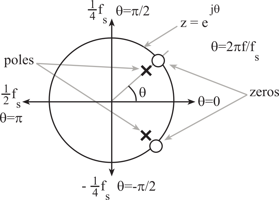
Figure M.6.10. Pole-zero plot of a 60 Hz digital notch filter.
The transfer function is
![]()
which can be put in standard form (i.e., with terms 1, z-1, z-2 ...)
![]()
The digital filter can be derived by taking the inverse Z-transform of the H(z) equation
y(n) = x(n) - 2cos(θ)x(n-1) + x(n-2) + 2αcos(θ)y(n-1) - α2y(n-2)
Sometimes we can choose fs and/or α to simplify the digital filter equation. For example, if we choose fs = 240 Hz, then the "cos(θ)" terms become zero. If we choose α = 7/8 then the fixed-point digital filter becomes:
y(n) = x(n) + x(n-2) - (49*y(n-2))/64
Another consideration for this type of filter is the fact that the gain in the pass bands is greater than one. The DC gain can be determined two ways. The first method is to use the H(z) transfer equation and set z=1. The H(z) transfer equation for the filter is
![]()
At z=1 this reduces to
![]()
The second method to calculate DC gain operates on the filter equation directly. In the first step, we set all x(n-k) terms in the filter to a single variable "x" and all y(n-k) terms in the filter to a single variable "y". Next, we solve for the DC gain, which is y/x.
y = x + x - (49*y)/64
This method also calculates the DC gain to be 128/113. We can adjust the digital filter so that the DC gain is exactly 1, by prescaling the input terms (x(n), x(n-1), x(n-2),...) by 113/128.
y(n) = (113*x(n) + 113*x(n-2) - 98*y(n-2))/128
int32_t x[3]; // MACQ for the ADC input data
int32_t y[3]; // MACQ for the digital filter output
void SysTick_Handler(void){
x[2] = x[1]; x[1] = x[0]; // shift data
y[2] = y[1]; y[1] = y[0];
x[0] = ADC_In(); // 0 to 4095
y[0] = (113*(x[0]+x[2])-98*y[2])/128; // filter output
Fifo_Put((int16_t)y[0]); // pass to foreground
}
Program M.6.5. If the sampling rate is 240 Hz, this filter rejects 60 Hz.
Since the gain of this filter is always less than or equal to one, the filter outputs will fit into 16-bit variables. However the intermediate term 113*(x[0]+x[2]) could be as large as 113*(4095+4095). 7bits*(12bits+12bits) is 20 bits, so 32-bit calculations are performed. The gain of this filter is shown in Figure M.6.11.
The "Q" of a digital notch filter is defined to be
![]()
where fc is the center or notch frequency, and ∆f frequency range where is gain is below 0.707 of the DC gain. For the filter in Figure M.6.11 the gains at 55 and 65 Hz are about 0.707, so its Q is 6.
: Use Figure M.6.11 to compare the filter Q of Program M.6.3 with the filter Q of Program M.6.5. Next, compare the execution speed of the two implementations. If you wished to remove 60 Hz and pass all other frequencies, which filter would you choose?
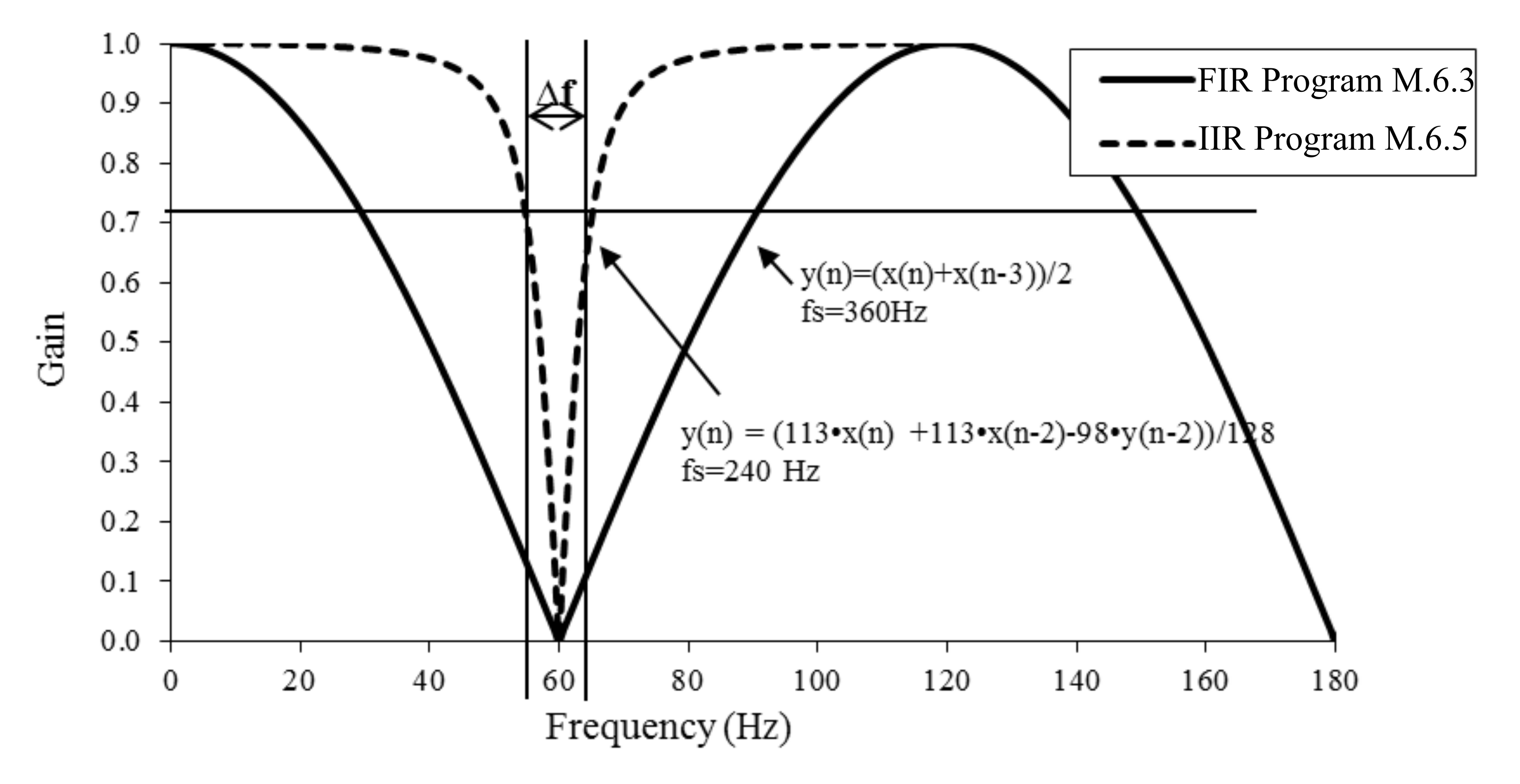
Figure M.6.11. Gain versus frequency response of two 60 Hz digital notch filters.
In this second example, we will design a band-pass filter that passes 50 to 100 Hz. In this example, signals exist from 0 to 240 Hz, so the sampling rate will be 480 Hz. Figure M.6.12 shows one possible pole-zero plot. First, we place the zeros so 50 to 100 Hz is passed, and other frequencies are rejected. As we increase the number of zeros, we can reduce the gain in places we wish to make the gain low, but the complexity of the filter increases. This filter with 8 zeros will have 8 x(n-k) terms in the equation. The idea is not to place any zeros in 50 to 100 Hz range, but place them around in the 0 to 50, and 100 to 240 regions. There is a spreadsheet (DigitalFilterDesign.xls **add link**) that you can manipulate to see how the filter shape responds to the placement of poles and zeros.
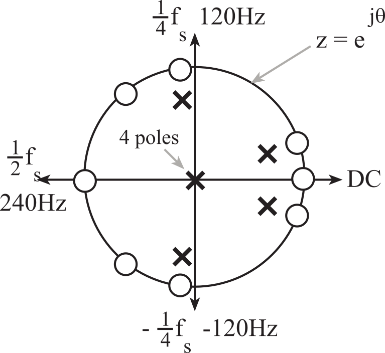
Figure M.6.12. Pole-zero plot of a 50 to 100 Hz digital band-pass filter.
Next, we place the poles. In this example, there will also be 8 poles. Placing the pole near a zero causes the gain to rise and fall quickly. Placing the pole away from a zero flattens the response. In this example, the zeros near 50 and 100 Hz have poles near them, and the others are away. The farthest away will be to place the poles at z=0. The transfer function is
![]()
The steps to derive the filter are the same as the last example. First, we multiply out the top and bottom expressions. Because the zeros are either at z=1, z=-1, or occur in complex conjugate pairs, the numerator will have real coefficients. Similarly, because the poles are either at z=0 or occur in complex conjugate pairs, the denominator will also have real coefficients. Next, we multiply the top and bottom by z-8, placing the transfer function in standard form. Next, we take the inverse transform to get the digital filter:
y(n) = a0*x(n) + a1*x(n-1) + a2*x(n-2) + a3*x(n-3) + a4*x(n-4) + a5*x(n-5)
+ a6*x(n-6) + a7*x(n-7) + a8*x(n-8) + b0*y(n-1) + b1*y(n-2) + b2*y(n-3) + b3*y(n-4)
Figure M.6.13 plots the gain of this filter. The details of these calculations can be found in the spreadsheet DigitalFilterDesign.xls. The coefficients are converted to binary fixed-point and implemented in Program M.6.6.
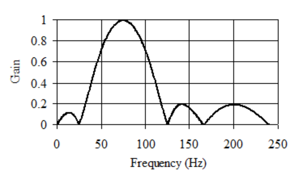
Figure M6.13. Gain versus frequency of a 50 to 100 Hz digital band-pass filter.
Typically, we design an IIR filter with an equal number of poles and zeros. If there are more zeros than poles, then filter is noncausal. For example, H(z)=z has one zero and no poles. The filter will be y(n) = x(n+1), which is noncausal. If there are more poles than zero, then filter will have a time delay or a very large gain. For example, H(z)=z-1 has one pole and no zeros. The filter will be y(n) = x(n-1).
const int32_t a[9]={2521,-1589,-617,-2296,0,2296,617,1589,-2521};
const int32_t b[4]={20220,-14068,9908,-3934};
int32_t x[9]; // MACQ for the ADC input data
int32_t y[5]; // MACQ for the digital filter output
void SysTick_Handler(void){
x[8] = x[7]; x[7] = x[6]; x[6] = x[5]; x[5] = x[4];
x[4] = x[3]; x[3] = x[2]; x[2] = x[1]; x[1] = x[0]; // shift data
y[4] = y[3]; y[3] = y[2]; y[2] = y[1]; y[1] = y[0];
x[0] = ADC_In(); // 0 to 4095
y[0] = (a[0]*x[0]+ a[1]*x[1]+ a[2]*x[2]+ a[3]*x[3]+ /* a[4]*x[4]+ */
a[5]*x[5]+ a[6]*x[6]+ a[7]*x[7]+ a[8]*x[8]+
b[0]*y[1]+ b[1]*y[2]+ b[2]*y[3]+ b[3]*y[4])/16384;
Fifo_Put((int16_t)y[0]); // pass to foreground
}
Program M.6.6. If the sampling rate is 480 Hz, this bandpass filter passes 50 to 100 Hz.
M.6.5. FIR Filter Design
In this section we will use the DFT as a general tool to design FIR filters. We begin by choosing the sampling rate, which must be larger than two times the largest signal frequency we wish to process. After we have chosen the sampling rate (e.g., 10 kHz), we will choose a FIR filter length (e.g., N=51). The ratio fs/N (e.g., 10 kHz/51 = 196 Hz) will determine the frequency resolution of the FIR filter design. The larger the N, the more gain points we can specify in the filter response, but the slower the filter will execute. Next, we plot or print the desired gain/phase versus frequency response. The magnitude of H(k) is selected to implement the desired gain versus frequency response. I.e., |H(k)| will be the filter gain at k*fS/N. The angle of H(k) is selected to implement the desired phase versus frequency response. I.e., angle[H(k)] will be the filter phase at k*fS/N. For frequencies above ½fs, we must make H(k) be the complex conjugate of the N-k term. This will guarantee that the inverse DFT of H(k) will yield real results. Let x(n) be the input (read from the ADC) and X(k) be the input in the frequency domain. Let y(n) be the FIR filter output, and let Y(k) be the FIR filter output in the frequency domain.
Y(k) = H(k) X(k)
y(n) = IDFT { H(z) DFT{x(t)} }
We take IDFT of the H(k) to get N FIR filter coefficients. Multiplication in the frequency domain is equivalent to convolution in the time domain. The FIR filter is the convolution of the data with the inverse transform of the desired filter.

Because there are a finite number of h(n) terms, the convolution is a finite sum
![]()
As an example, we will design a digital filter for a hearing aid that accentuates high frequencies. The input is audio with frequency components from 100 Hz to 5 kHz. We will make the gain equal to 5 for frequencies 2 to 5 kHz. For the lower audio frequencies make the gain equal to 1. We choose the sampling rate at twice the maximum frequency of the input or fs = 10 kHz. Next, we choose a filter size. The larger N, the better the actual filter will match our desired response, but the slower it will execute. For this solution, we could have chosen any size from 32 to 64 and obtained similar results. To preserve the shape of the audio signals, we will implement linear phase. The desired filter gain is shown as Figure M.6.14 and Table M.6.2. The lines in the figure are the desired filter gain, and the dots will be the actual gain as implemented by the fixed-point math in Program M.6.7. The details of this filter design can be found in the spreadsheet FIRdesign51.xls **add link**
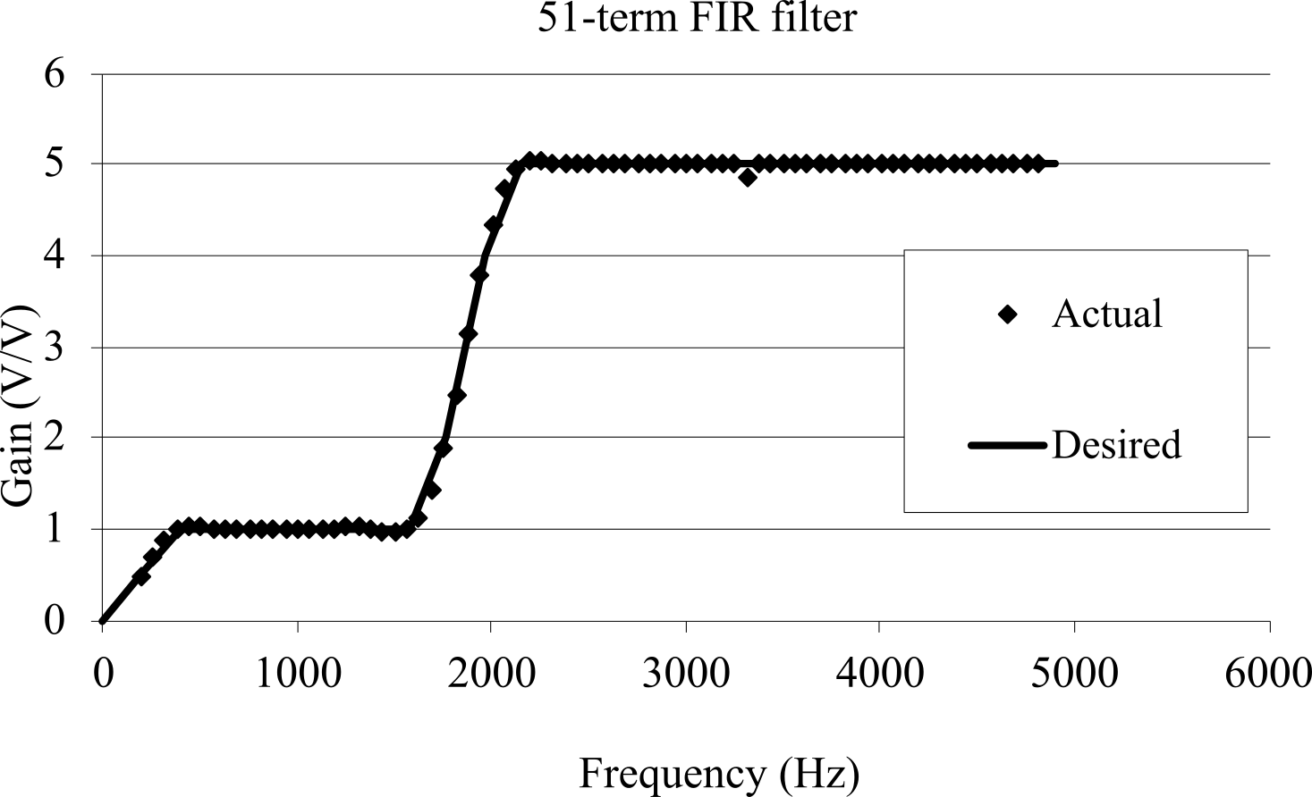
Figure M.6.14. Desired and actual filter responses. This is H.
The H(N-k) values must be the complex conjugates of H(k). Because the negative frequencies in Table 6.3 are complex conjugates of the positive frequencies, h(n) will be real. Next, we scale the h(n) values to make 51 fixed-point coefficients h[51]. For example, the first term h(1) is -0.000457, which will be approximated in fixed-point as -7/16384. In summary, the h[51] coefficients are the IDFT of the values in Table M.6.3 multiplied by 16384 and rounded to an integer.
const int32_t h[51]={0,-7,-45,-64,5,78,-46,-355,-482,-138,329,
177,-722,-1388,-767,697,1115,-628,-2923,-2642,1025,4348,1820,-8027,
-19790,56862,-19790,-8027,1820,4348,1025,-2642,-2923,-628,1115,697,
-767,-1388,-722,177,329,-138,-482,-355,-46,78,5,-64,-45,-7,0};
|
k |
f (Hz) |
Mag(H(k)) |
Angle(H(k)) |
|
k |
f (Hz) |
Mag(H(k)) |
Angle(H(k)) |
|
0 |
0.00 |
0.00 |
0.00 |
|
13 |
2549.02 |
5.00 |
-40.04 |
|
1 |
196.08 |
0.50 |
-3.08 |
|
14 |
2745.10 |
5.00 |
-43.12 |
|
2 |
392.16 |
1.00 |
-6.16 |
|
15 |
2941.18 |
5.00 |
-46.20 |
|
3 |
588.24 |
1.00 |
-9.24 |
|
16 |
3137.25 |
5.00 |
-49.28 |
|
4 |
784.31 |
1.00 |
-12.32 |
|
17 |
3333.33 |
5.00 |
-52.36 |
|
5 |
980.39 |
1.00 |
-15.40 |
|
18 |
3529.41 |
5.00 |
-55.44 |
|
6 |
1176.47 |
1.00 |
-18.48 |
|
19 |
3725.49 |
5.00 |
-58.52 |
|
7 |
1372.55 |
1.00 |
-21.56 |
|
20 |
3921.57 |
5.00 |
-61.60 |
|
8 |
1568.63 |
1.00 |
-24.64 |
|
21 |
4117.65 |
5.00 |
-64.68 |
|
9 |
1764.71 |
2.00 |
-27.72 |
|
22 |
4313.73 |
5.00 |
-67.76 |
|
10 |
1960.78 |
4.00 |
-30.80 |
|
23 |
4509.80 |
5.00 |
-70.84 |
|
11 |
2156.86 |
5.00 |
-33.88 |
|
24 |
4705.88 |
5.00 |
-73.92 |
|
12 |
2352.94 |
5.00 |
-36.96 |
|
25 |
4901.96 |
5.00 |
-77.00 |
Table M.6.2. Desired filter response. This is H.
Program M.6.7 shows the implementation of this FIR filter. There are 100 µs for each sample (ADC, filter, and DAC). We will implement the MACQ using two copies of the data. We could add this filter to the audio recordings from a microphone (add link to microphone**.
int16_t Data[102]; // two copies
int16_t *Pt; // pointer to current
void Filter_Init(void){
Pt = &Data[0];
}
// calculate one filter output
// called at sampling rate
// Input: new ADC data
// Output: filter output, DAC data
int16_t Filter_Calc(int16_t newdata){
int i; int32_t sum; int16_t *pt,*apt;
if(Pt == &Data[0]){
Pt = &Data[50]; // wrap
} else{
Pt--; // make room for data
}
*Pt = *(Pt+51) = newdata; // two copies
pt = Pt; // copy of data pointer
apt = h; // pointer to coefficients
sum = 0;
for(i=51; i; i--){
sum += (*pt)*(*apt);
apt++;
pt++;
}
return sum/16384;
}
Program M.6.7. 51-term FIR filter
: How can we prove the software in Program M.6.7 cannot overflow?
: Can you think of a way to reduce the number of multiplies in Program M.6.7 while still performing the exact same filter?
M.7. Student's t-test
M.7.1. Unpaired (two-sample) Student's t-test
We can use the Student's t-test to determine if two measurement sets have different means. More specifically, the unpaired t method tests the null hypothesis that the population means related to two independent, random samples from an approximately normal distribution are equal. We use the unpaired method when the ith data point in the first measurement set is not related to the ith data point in the second measurement set. In general, we cannot prove two means are equal. We can however state, "the data cannot prove the means are different".
Consider an instrument that measures temperature. If we wanted to measure temperature resolution, we would take a set of measurements with a known input temperature of T1. Then we would increase the temperature to T1+DT. If the system can reliably detect the change in temperature, then we would claim the measurement resolution is less than or equal to DT, as shown in Figure M.7.1.

Figure M.7.1. Resolution is the smallest change in input that can be reliably detected.
Resolution is defined as the smallest change that can be reliably detected. We can use the student's t-test to define "reliably detected".
If a random variable, X, is normally distributed with a mean is m and a standard deviation of s, then the probability that it falls between ±1 s is 68 %. I.e.,
P(m-s < X < m+s) = 0.68
Similarly,
P(m-1.96s < X < m+1.96s) = 0.95
P(m-2s < X < m+2s) = 0.954
P(m-2.58s < X < m+2.58s) = 0.99
P(m-3s < X < m+3s) = 0.9997
The square of the standard deviation is called variance, s2. In most situations, we do not know the mean and standard deviation, so we collect data and estimate them
![]()
The N-1 term is used in the calculation of S because there are N-1 degrees of freedom. These expressions are unbiased estimates of m and s, meaning as the sample size increases the estimates approach truth. Formally, we say
![]()
For example, we collect two sets of data, as plotted in Figure M.7.1, and we want to know if the means of two sample sets are different. To use the Student's t test we need to make the following assumptions:
1) the errors in one data set are independent (not correlated to) the errors in the other data set;
2) the errors in each data sample are independent (not correlated to) the errors in other data within that set;
3) the errors are normally distributed;
4) the variance is unknown;
5) the variances in the two sets are equal.
Consider the measurements in the two data sets as the sum of the true value plus an error:
X0i = m0 + e0i
X1i = m1 + e1i
Assumption 1 states that e0i are not correlated to e1i. Assumption 2 states that e0i are not correlated to e0j and e1i are not correlated to e1j. Thermal noise will satisfy these assumptions. We employ a test statistic to test the hypothesis H0: m0= m1. First, we estimate the means and variances of the data (assuming equal sized samples)

From these, we calculate the test statistic t:
![]()
There are formulas for t if the size of the two data sets are not equal, but only the simple case of equal data sizes are included in this section. The two sets of data, together, have 2N-2 degrees of freedom. The Student's t table, shown as Table M.7.1, has two dimensions. In the vertical direction, we specify the degrees of freedom, df. For example, if there are 10 data points in each data set, then df equals 18. In the horizontal direction we select the probability of being correct. For example, if we wish to be 99% sure of the test, then we select the 99% column. Selecting the row and the column allows us to pick a number threshold. For example, the number in the df=18 row, confidence=99% column is 2.878. This means if H0 is true, then
Probability of t < -2.878 = 0.005 and Probability of t > 2.878 = 0.005
Therefore
Probability of -2.878 < t < 2.878 = 0.99 (confidence interval of 99%)
If we collect data and calculate t such that the test statistic t is greater than 2.878 or less than -2.878, then we claim "we reject the hypothesis that the means are equal (p<0.01)". If the test statistic t is between -2.878 and 2.878, we do not claim the hypothesis to be true. In other words, we have not proven the means to be equal. Rather, we say "we do not reject the hypothesis that the means are equal".
|
confidence |
80% |
90% |
98% |
99% |
99.8% |
99.9% |
|
df p= |
0.10 |
0.05 |
0.01 |
0.005 |
0.001 |
0.0005 |
|
8 |
1.397 |
1.860 |
2.896 |
3.355 |
4.501 |
5.041 |
|
9 |
1.383 |
1.833 |
2.821 |
3.250 |
4.297 |
4.781 |
|
10 |
1.372 |
1.812 |
2.764 |
3.169 |
4.144 |
4.587 |
|
11 |
1.363 |
1.796 |
2.718 |
3.106 |
4.025 |
4.437 |
|
12 |
1.356 |
1.782 |
2.681 |
3.055 |
3.930 |
4.318 |
|
13 |
1.350 |
1.771 |
2.650 |
3.012 |
3.852 |
4.221 |
|
14 |
1.345 |
1.761 |
2.624 |
2.977 |
3.787 |
4.140 |
|
15 |
1.341 |
1.753 |
2.602 |
2.947 |
3.733 |
4.073 |
|
16 |
1.337 |
1.746 |
2.583 |
2.921 |
3.686 |
4.015 |
|
17 |
1.333 |
1.740 |
2.567 |
2.898 |
3.646 |
3.965 |
|
18 |
1.330 |
1.734 |
2.552 |
2.878 |
3.610 |
3.922 |
|
19 |
1.328 |
1.729 |
2.539 |
2.861 |
3.579 |
3.883 |
|
20 |
1.325 |
1.725 |
2.528 |
2.845 |
3.552 |
3.850 |
|
21 |
1.323 |
1.721 |
2.518 |
2.831 |
3.527 |
3.819 |
|
22 |
1.321 |
1.717 |
2.508 |
2.819 |
3.505 |
3.792 |
|
23 |
1.319 |
1.714 |
2.500 |
2.807 |
3.485 |
3.767 |
|
24 |
1.318 |
1.711 |
2.492 |
2.797 |
3.467 |
3.745 |
|
25 |
1.316 |
1.708 |
2.485 |
2.787 |
3.450 |
3.725 |
|
26 |
1.315 |
1.706 |
2.479 |
2.779 |
3.435 |
3.707 |
|
27 |
1.314 |
1.703 |
2.473 |
2.771 |
3.421 |
3.690 |
|
28 |
1.313 |
1.701 |
2.467 |
2.763 |
3.408 |
3.674 |
|
29 |
1.311 |
1.699 |
2.462 |
2.756 |
3.396 |
3.659 |
|
30 |
1.310 |
1.697 |
2.457 |
2.750 |
3.385 |
3.646 |
|
40 |
1.303 |
1.684 |
2.423 |
2.704 |
3.307 |
3.551 |
|
50 |
1.299 |
1.676 |
2.403 |
2.678 |
3.261 |
3.496 |
|
60 |
1.296 |
1.671 |
2.390 |
2.660 |
3.232 |
3.460 |
|
80 |
1.292 |
1.664 |
2.374 |
2.639 |
3.195 |
3.416 |
|
100 |
1.290 |
1.660 |
2.364 |
2.626 |
3.174 |
3.390 |
|
120 |
1.289 |
1.658 |
2.358 |
2.617 |
3.160 |
3.373 |
|
∞ |
1.282 |
1.645 |
2.326 |
2.576 |
3.090 |
3.291 |
Table M.7.1. Student's t distribution table.
M.7.2. Paired Student's t-test
You use the paired t-test when there is one measurement variable and two nominal variables. A measurement variable is something we measure resulting in a number, like distance, temperature, pressure, or speed. A nominal variable is described as a word or name, such as Bill, Jon, and Sam. The first nominal variable is usually the names or identity of different animals or patients. The second nominal variables has only two values, signifying either spatial or temporal information such as "left right" or "before after".
An example would be the time to run 50 meters before and after drinking a cup of coffee. For each person, there would be two measurements, the time to run 50 meters before the coffee and another time to run after the coffee. We expect the people to vary widely in their performance, so if the coffee decreased their mean performance by 5 percent, it would take a very large sample size to detect this difference if the data were analyzed using a Student's t-test. Using a paired t-test has much more statistical power when the difference between groups is small relative to the variation within groups.
The paired t-test is only appropriate when there is just one measurement for each combination of the nominal values. For the coffee example, that would be one measurement of time on each person before drinking coffee, and one measurement after drinking coffee. If you had multiple measurements you would do a two-way anova with replication.
The null hypothesis is that the mean difference between paired observations is zero. This is mathematically equivalent to the null hypothesis of an unpaired t-test, but because of the data are paired, the null hypothesis of a paired t-test is usually expressed in terms of the mean difference. The paired t-test assumes that the differences between pairs are normally distributed. The difference between the observations is calculated for each pair, and the mean and standard error of these differences are calculated. Dividing the mean by the standard error of the mean yields a test statistic, t, that is t-distributed with degrees of freedom equal to one less than the number of pairs. There are two data sets, which are the sum of the true value plus an error:
X0i = m0 + e0i
X1i = m1 + e1i
First, we calculate the difference between each pair
Yi = X1i - X0i
Next, we calculate the average and standard deviation of the differences
![]()
The standard error is
![]()
The t-statistic is
![]()
and the degrees of freedom are N-1.
As an example, a measurement is taken before and after a treatment on 9 patients.
|
Subject |
Before |
After |
Difference |
|
1 |
31 |
30 |
-1 |
|
2 |
24 |
20 |
-4 |
|
3 |
34 |
23 |
-11 |
|
4 |
39 |
31 |
-8 |
|
5 |
30 |
22 |
-8 |
|
6 |
25 |
26 |
1 |
|
7 |
39 |
33 |
-6 |
|
8 |
40 |
33 |
-7 |
|
9 |
29 |
23 |
-6 |
Table M.7.2. Example experiment collecting measurements on patients before and after treatment.
The average difference is -5.56, the standard deviation of the difference is 3.71, the standard error is 1.24, the t-statistic is -4.49, and the degree of freedom is 8. We find the t=4.5, df=8 as a confidence 99.8% in the table, so we say the null hypothesis of no difference between the means is rejected (p<0.002).