Chapter 10. Examples

Table of Contents:

10.1. Measurement of Temperature
10.2. Electrocardiogram
10.3. Stepper Motor Robot
10.4. Buddy Follower Robot using Fuzzy Logic
10.5. Autonomous Racing Robot using Performance Maps
10.6. Lab 10 Audio Communication

We introduced the design process back in Section 1.4. The Design Process. In this chapter, we will present the designs of five embedded systems. The first example is a quantitative measurement of temperature, the second example is a qualitative measurement of electrocardiogram signals, and the remaining examples involve robots.

10.1. Measurement of Temperature

Example 10.1. Design an instrument that measures temperature with a range of 0 to 40˚C, and a resolution is 0.01˚C. The frequency range of interest is 0 to 20 Hz.

Solution: The first decision to make is the choice of transducer. The RTD has a linear resistance versus temperature response. RTDs are expensive, but a good choice for ease of calibration, interchangeability, and accuracy. Thermocouples are inexpensive and a good choice for large temperature ranges, harsh measurement conditions, fast response time, interchangeability, and large temperature ranges. Interchangeability means we can buy multiple transducers, and they will all have similar temperature curves. Thermistors will be used in this design because they are inexpensive and have better sensitivity than RTDs and thermocouples. A thermometer built using a thermistor will be harder to mass-produce because each transducer must be separately calibrated to create an accurate measurement. From a first glance, we might expect a 12-bit ADC will generate a temperature resolution of 0.01 ˚C. Recall that range equals resolution times precision. On the other hand, because the thermistor is nonlinear, we will need to verify the resolution specification is met. Figure 10.1.1 shows the block diagram of the instrument, which also illustrates the data flow in our system.

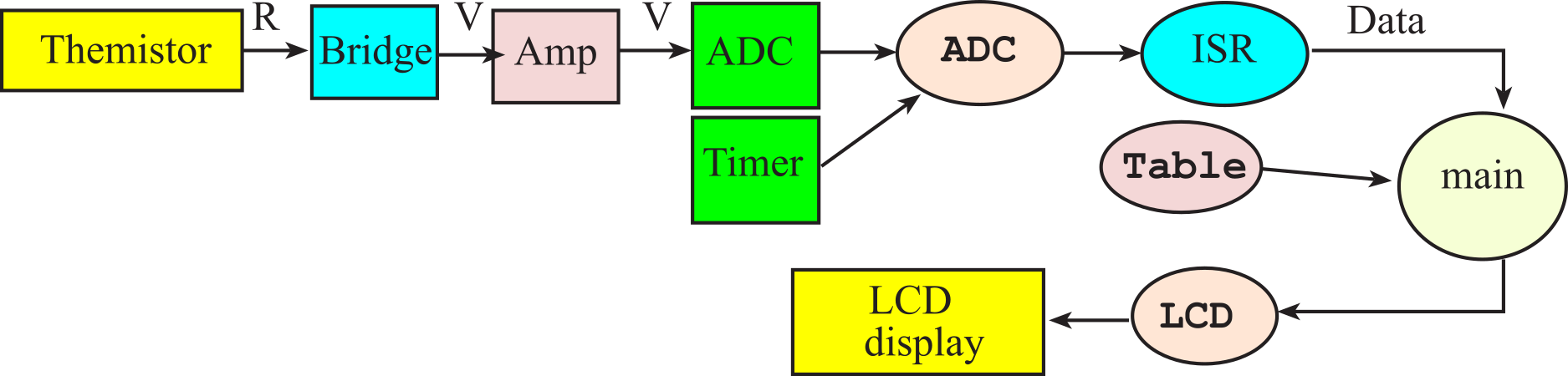
Figure 10.1.1. Data flow graph of a temperature measurement system using a thermistor.

The resistance bridge is a classic means to convert resistance to voltage. Table 10.1.1 is used during the design phase to show the signal values as they transverse the system. A +2.50 V reference drives the bridge. The value of resistor R₁ is chosen to eliminate errors due to self-heating the thermistor (100 kΩ). The first two columns of Table 10.1.1 give the thermistor calibration. Since we will be using rail-to-rail electronics, we need to have all voltages between the 0 to +3.3 V range. We can make the bridge output (V₁-V₂) positive by selecting the value of resistor R₂ less than the thermistor resistance at the maximum temperature (56.4 kΩ). For this thermistor, R₂ is selected at 51 kΩ because it is a standard resistor less than 56.4 kΩ. Next, we choose the gain of the amplifier to map the minimum temperature into the +3.3V limit of the ADC. Using an INA122, a gain resistor of 330 kΩ creates the desired gain of 5.61. Since the thermistor is nonlinear, we will tabulate explicit values to determine the ADC precision required (Table 10.1.2). There are two possible approaches to the design of the amplifier. If we use an instrumentation amp, the input impedance will be large enough not to affect the bridge. If we use a single op amp differential amp, then the amplifier will load the bridge and affect the bridge response. In this system, the instrumentation amp will be used. The first two columns of Table 10.1.1 show the resistance temperature calibration of the thermistor. The third column, V₁, is the voltage across the thermistor. The fourth column is the output of the bridge, V₁-V₂. V_out, the output of the instrumentation amp, is shown in the fifth column. The ADC value gives the digital output of a 12-bit converter, and the last column will be calculated by our software as a decimal fixed-point with resolution 0.01 ˚C. We use this table in two ways. Initially, we use the theoretical values to design the electronics and software. During the implementation phase, we substitute resistors with standard values to bring down the cost. During the testing phase, we measure actual values to verify proper operation. Measured values for the last two columns will be stored in software as a calibration table. To measure temperature, the software measures the ADC value and then uses a table look-up and linear interpolation to get the decimal fixed-point temperature (last column). The fixed-point number is output to an LCD display.

Observation: There is an Excel worksheet named Therm12.xls that was used to create this design.

T (°C)	R_t (kΩ)	V₁ (V)	V₁-V₂ (V)	V_out (V)	ADC	T (0.01˚C)
0.00	234.312	0.832	0.587	3.291	4083	0
8.00	170.637	0.666	0.421	2.361	2929	800
16.00	126.466	0.530	0.285	1.600	1985	1600
24.00	95.253	0.421	0.177	0.990	1228	2400
32.00	72.818	0.335	0.091	0.508	630	3200
40.00	56.436	0.268	0.023	0.131	162	4000

Table 10.1.1. Signals as they pass through the temperature data acquisition system.

To prevent noise in the ADC samples, the noise must be less than the resolution. Using Table 10.1.2, the needed resolution of V₁-V₂ is about 0.1 mV. Adding a safety factor of ½ gives the maximum allowable noise referred to the input of the INA122 is 50 µV, in the frequency range 0 to 20 Hz:

amplifier noise ≤ = 50 µV

A two-pole low pass analog filter (Section 6.5.2. Butterworth Filters) is used to pass the temperature signal having frequencies from 0 to 20 Hz, reject noise having frequencies above ½f_s. To prevent aliasing, Z must be less than the ADC resolution for all frequencies larger than or equal to ½f_s. As an extra measure of safety, we make the amplitude less than 0.5 ∆z for frequencies above ½f_s . Thus,

| Z | < 0.5 ∆z = 3.3V/8192 ≈ 0.4 mV

The effective output impedance of the bridge is less than 234 kΩ. The input impedance of the differential amp must be high enough to not affect the 12-bit ADC conversion. The input impedance of the INA122 is 10 GΩ.

Zin > 234 kΩ * 2ⁿ⁺¹= 234 kΩ * 8192 =2 GΩ

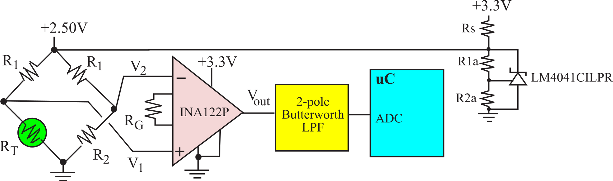
Figure 10.1.2. Amplifier and low pass filter.

To determine the resolution we work backwards, as illustrated in Table 10.1.2. The basic approach to verifying the temperature resolution is to work backwards through the circuit, showing that a change in ADC value of 1 corresponds to a temperature change of 0.02 ˚C.

ADC	V₃ (V)	V₁-V₂ (V)	V₁ (V)	R_T (kΩ)	T (°C)	∆T (˚C)
4095	3.299	0.5885	0.8332	234.9549	-0.067
4094	3.298	0.5884	0.8331	234.8941	-0.061	0.0063
2048	1.650	0.2943	0.5390	129.1981	15.414
2047	1.649	0.2942	0.5389	129.1542	15.423	0.0093
1	0.001	0.0001	0.2449	51.0332	43.276
0	0.000	0.0000	0.2447	51.0000	43.297	0.0214

Table 10.1.2. Equations calculated in reverse to show that the resolution meets the design specification.

There are three possible approaches to converting ADC sample to temperature (the last two columns of Table 10.1.1). First, we could fit the transfer function to a polynomial equation and save the coefficients of that equation as the calibration file. This approach performs well for simple situations. A plot of this data is shown as Figure 10.1.3. Second, we could calculate the temperature output for each possible ADC and save it in a 4096-entry lookup table. This conversion is fast because we just need to use the ADC data to index into the big table. This method is fast, but requires a lot of ROM. The third approach, shown in Program 10.1.1, uses a table of paired (ADC,T) data. These points are determined from experimental calibration. To find the corresponding temperature for a given ADC value, the program first searches the table for a pair of ADC-values that surround the input. Extra entries were added at the beginning and end of the table to guarantee the search step will always be successful. Then, it uses linear interpolation to calculate the temperature, given the 53 entries in the table and the ADC input. The output result is a fixed-point number with a resolution of 0.01 ˚C.

Typically, the resolution of this thermometer will depend on analog noise rather than ADC resolution. The accuracy will depend on both resolution and calibration drift. Drift is defined as a change over time of the data in Figure 10.1.3 and the numbers in Program 10.1.1. For software that converts the ADC sample, see Section M.1. Interpolation.

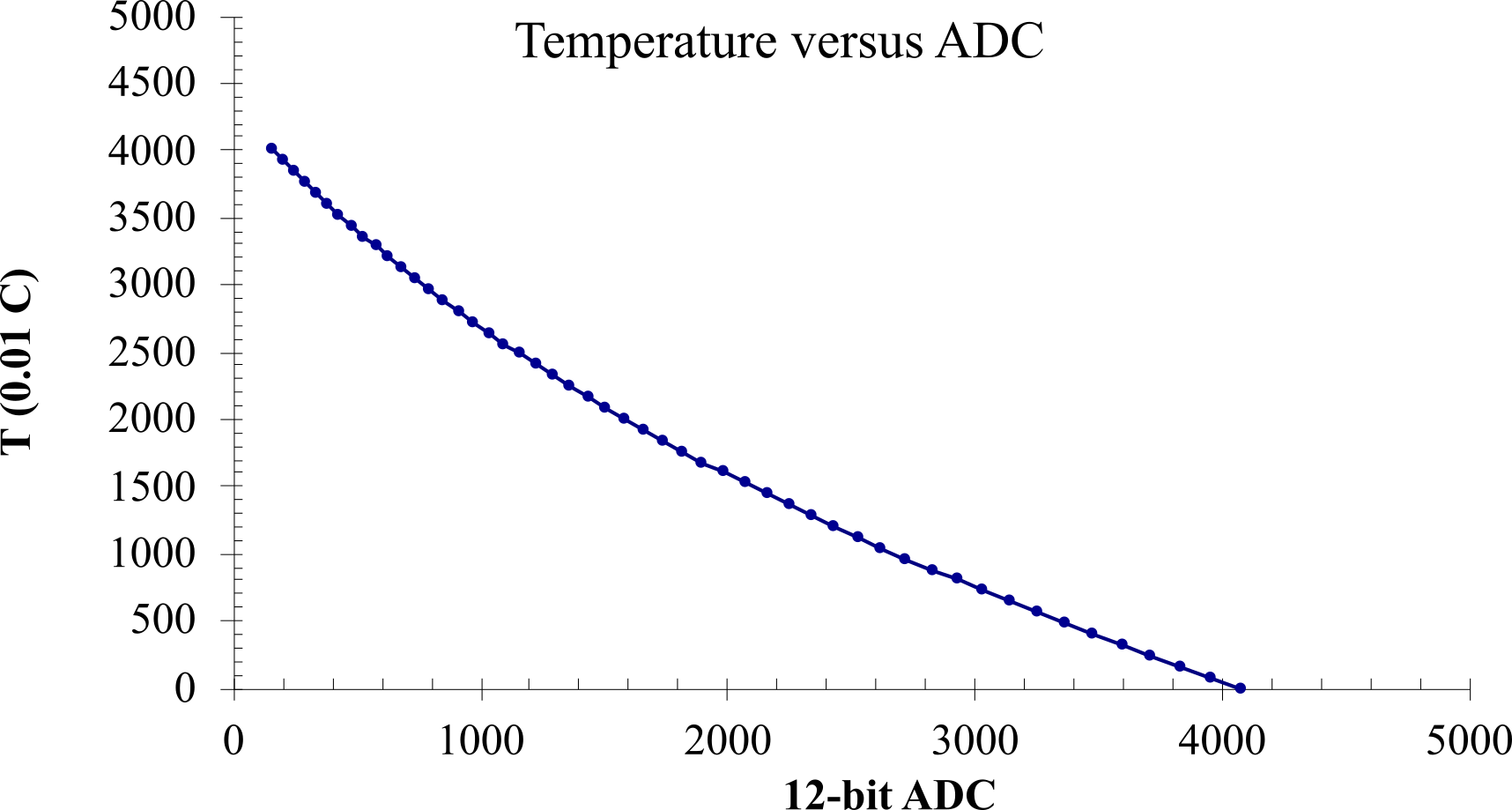
Figure 10.1.3. Transfer function between sampled 12-bit ADC and fixed-point temperature.

The calibration data in Adata and Tdata are stored in flash ROM. In general, we perform time-critical tasks like ADC sampling in the background, and noncritical functions like conversion to temperature and LCD output in the foreground. Therefore, the interrupt service routine passes the measured temperature to the foreground through a FIFO queue, and the main program has the responsibility of outputting the result to the LCD.

// table of multiple unsigned (x,y), piece-wise linear function

int32_t const Adata[53]={0,162,203,246,290,335,381,429,477,527,578,

630,684,738,795,852,911,971,1033,1096,1161,

1228,1296,1365,1437,1510,1584,1661,1739,1819,1901,

1985,2070,2158,2247,2338,2432,2527,2625,2724,2826,

2929,3035,3143,3253,3365,3479,3596,3714,3835,3958,4083,4096

};

int32_t const Tdata[53]={4000,4000,3920,3840,3760,3680,3600,3520,3440,3360,3280,

3200,3120,3040,2960,2880,2800,2720,2640,2560,2480,

2400,2320,2240,2160,2080,2000,1920,1840,1760,1680,

1600,1520,1440,1360,1280,1200,1120,1040,960,880,

800,720,640,560,480,400,320,240,160,80,0,0

};

Program 10.1.1. Calibration data for thermistor.

: What would be the temperature resolution if the ADC precision were decreased from 12 to 8 bits?

To measure temperature resolution, we use the student's t-test to determine if the system can detect the change. See Section M.7.1. Unpaired (two-sample) Student's t-test.

10.2. Electrocardiogram

Example 10.2. Design a system to measure electrical activity in the heart. We wish to measure heart rate.

Solution: Biopotentials are important measurements in many research and clinical situations. Biopotentials are electric voltages produced by individual cells and can be measured on the skin surface. The status of the heart, brain, muscles, and nerves can be studied by measuring biopotentials. Electrodes, which are attached to the skin, interface the machine to the body. Electronic instrumentation amplifies and filters the signal. For example, Figure 10.2.1 shows a normal Lead II electrocardiogram, or EKG, which is measured with the positive terminal attached to the left arm, the negative terminal attached to the right arm, and ground connected to the right leg. Each wave represents one heartbeat, and the shape and rhythm of this wave contains a lot of information about the health and status of the heart.

Figure 10.2.1. Normal II-lead electrocardiogram.

There are two types of electrodes used to record biopotentials. Nonpolarizable electrodes like silver/silver chloride involve the following chemical reaction in the electrode at the electrode/tissue interface:

AgCl + e^- ↔ Ag + Cl^-

A nonpolarizable electrode has a low electrical impedance because electrons can freely pass the electrode/tissue interface. In the electrode, current flows by moving electrons, but in the tissue current flows by physical motion of charged ions (e.g., Na⁺, K⁺ and Cl^-). A silver/silver chloride electrode does include a half-cell potential of 0.223 V, but since biopotentials are always measured with two electrodes, these half-cell potentials cancel. On the other hand, if you tried to use these electrodes to measure DC voltages, then the above chemical reaction would saturate and fail. Fortunately, biopotentials are produced by muscles and nerves are AC only and have no DC component.

Polarizable electrodes, made from metals like platinum gold or silver, have a high electrical impedance because electrons cannot freely pass the electrode/tissue interface. Charge can develop at the electrode/tissue interface effectively creating a capacitive barrier. Displacement current can flow across the capacitor, allowing the AC biopotentials to be measured by the electronics. The metallic electrodes also include half-cell potential, but again, these potentials will be cancelled.

Ag⁺ + e^- ↔ Ag

The graphical display of EKG versus time is an example of a qualitative data acquisition system. The measurement of heart rate is quantitative. The parameters of an EKG amplifier include: high input impedance (larger than 1 MΩ), high gain, 0.05 to 100 Hz bandpass filter and good common mode rejection ratio. The EKG signal is about ±1 mV, so an overall gain of about 2000 will produce a range of 0 to +3.3V on V₃. This EKG amp (Figure 10.2.2) begins with a preamp stage having a good CMRR, high input impedance, and a gain of 10. If the system is battery operated, then it does not need a third or ground electrode. Pin 5 of the AD627 is the analog ground, which in this circuit is the 1.233 V reference voltage. The AD627 is rail-to-rail. A 0.05 Hz passive high pass filter is created by R₄ and C₄. Low-leakage capacitors for C₁, C₂, and C₄ are critical for elimination of DC offset drift. C0G ceramic capacitors are needed for all capacitors except C3 and C5. The remaining gain is performed with a non-inverting amplifier (U2a). The LPF is implemented as a 2-pole Butterworth LPF. The 153 Hz cutoff was chosen because it is greater than 100Hz and can be implemented with standard components. If the signal V₁ saturates, you can reduce the gain of the preamp and increase the gain of the amp.

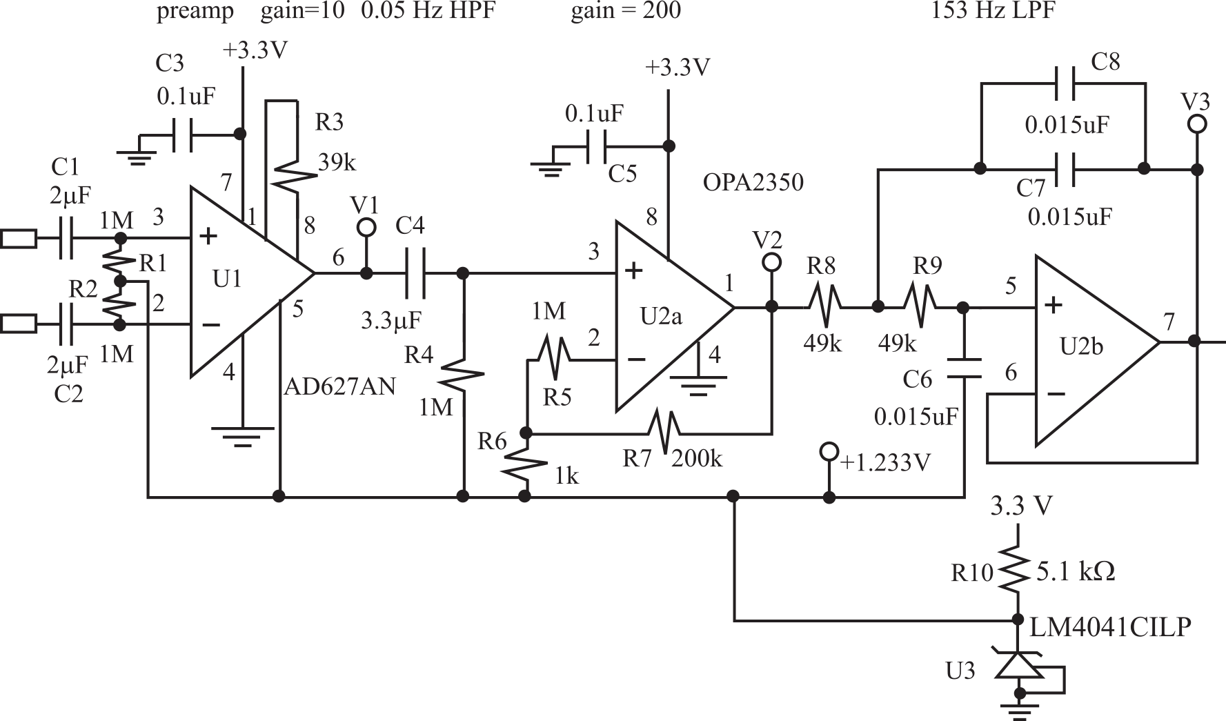
Figure 10.2.2. A battery-power EKG instrument.

Program 10.2.1 shows the real-time data acquisition and 60 Hz digital notch filter. The design of digital filters can be found in Section M.6. Digital Filter Design). The ADC sampling occurs in the background and the data are passed to the foreground using a FIFO queue. The large pulse in the EKG, originating from the contraction of the ventricles, is called the R-wave and it occurs once a heartbeat. Program 10.2.2 shows the foreground process, where there are four calculation steps performed on the EKG data. A low pass filter followed by a high pass filter capture a narrow band of information around 8 Hz. The square function calculates power and the 200 ms wide moving average gives an output very specific for the R-wave. Hysteresis is implemented with two thresholds. A heartbeat is counted (RCount++) when the moving average goes below the LOW threshold, then above the HIGH threshold. This software uses a combined frequency-period method to calculate heart rate. The algorithm to measure heart rate searches for R-waves in a 5-second interval. Rfirst is the time (in 1/120 sec units) of the first R-wave and Rlast is the time (also in 1/120 sec units) of the last R-wave. (RCount-1) is the number of beat-to-beat intervals between Rfirst and Rlast. The number 7200 is the conversion between the sample period (1/120 sec) and one minute. For example, at 72 BPM, there will be 6 R-waves detected in the 5-second interval, making (Rcount-1) equal to 5 and the difference Rlast-Rfirst will be 500. For more information on EKG systems, see Webster's book Medical Instrumentation, published by Wiley 2020, or Pan and Tompkins, "A Real-Time QRS Detection Algorithm," IEEE Transactions on Biomedical Engineering, pp. 230-236, March 1985.

Warning: If you are going to build an EKG, please have a trained engineer verify the safety of your hardware and software before you attach your machine to people.

void SysTick_Handler(void){ int16_t data;

data = ADC_In()-2048; // twos complement

Fifo_Put(data); // pass to foreground

}

Program 10.2.1. Real-time sampling of EKG (see program 8.8), sampled at 120 Hz.

int16_t Data; // ADC sample, -2048 to +2047, 12-bit signed ADC sample

int16_t x[50]; // sampled EKG, 120Hz

int16_t y[50]; // low pass filter, 120Hz

int16_t z[50]; // high pass filter, 120Hz

int16_t w[50]; // squared result, R-wave power, 120Hz

int16_t Rwav; // moving average of R-wave power, energy

uint16_t n=25; // 25,26, ..., 49

uint16_t Trigger;

#define HIGH 100 // trigger when over this

#define LOW 20 // reset when under this

uint16_t Rcount; // number of R-waves

uint16_t Rfirst; // time of first R-wave

uint16_t Rlast; // time of last R-wave

uint16_t HeartRate; // units bpm

int main(void) { uint16_t time; // units 1/120sec

int16_t lpfSum=0,hpfSum=0,RwavSum=0;

ADC_Init();

Fifo_Init();

Trigger =0; // looking for HIGH

SysTick_Init(); // 120 Hz sampling

while(1) {

Rcount = 0;

Rlast = 0;

for(time=0;time<600;time++){ // 120 Hz, every 5 second

while(Fifo_Get(&Data)){}; // Get data from background thread

Plot(Data); // draw voltage versus time plot

n++; if(n==50) n=25;

x[n] = x[n-25] = Data; // new data

lpfSum = lpfSum+x[n]-x[n-4];

y[n] = y[n-25] = lpfSum/4; // Low Pass Filter

hpfSum = hpfSum+y[n]-y[n-10];

z[n] = z[n-25] = y[n]-hpfSum/10; // High Pass Filter

w[n] = w[n-25] = (z[n]*z[n])/10; // Power calculation

RwavSum = RwavSum+w[n]-w[n-24]; // 200ms wide moving average

Rwav = RwavSum/24;

if(Trigger){

if(Rpow<LOW){

Trigger = 0; // found low

}

} else{

if((Rpow>HIGH)&&((time-Rlast)>30)){ // max HR= 240bpm

Trigger = 1; // found high

if(Rcount){

Rlast = time; // mark time of last R-wave, units 1/120sec

} else{

Rfirst = time; // mark time of first R-wave

}

Rcount++;

}

if(Rcount>=2){

HeartRate = (7200*(int32_t)(Rcount-1))/(int32_t)(Rlast-Rfirst);

} else{

HeartRate = 0;

}

Output(HeartRate); // display results

}

Program 10.2.2. Measurement of heart rate.

: What is the theoretical heart rate resolution of this approach when the HR is 60 BPM?

Common error: There are two reasons for EKG circuits to fail. The first poor contact between the skin and electrode causing a reduction in CMRR, and second is resistive leakage in capacitors C₁ C₂ C₄. Clean the skin well, use new electrodes and select a high quality capacitors.

10.3. Stepper Motor Robot

Example 10.3. Design an autonomous robot using a FSM and stepper motors. Make the robot avoid walls.

Video 10.3.1. Robot Car - Problem Statement and STG

Solution: We choose a stepper motor according to the speed and torque requirements of the system. A stepper with 200 steps/rotation will provide a very smooth rotation while it spins. Just like the DC motor, we need an interface that can handle the currents required by the coils. We can use a L293 to interface either unipolar or bipolar steppers that require less than 1 A per coil. In general, the output current of a driver must be large enough to energize the stepper coils. We control the interface using an output port of the microcontroller, as shown in Figure 10.3.1. Motors require interface circuits, like the L293, because of the large currents required for the motor. Furthermore, most motors will require more current than the USB or LaunchPad can supply. In this system the motors are powered directly from an 8.4V battery. Motor current flows from the battery to the L293, out 1Y, across the coil of the stepper motor, into the 2Y-pin of the L293, and finally back to the battery. Notice the motor currents do not flow across the LaunchPad or in/out the USB. The circuit shows the interface of two bipolar steppers, but the unipolar stepper interface is similar except there would be a direct connection of +8.4V to the motor (see Figure 10.3.2). The front of the robot has two bumper switches. The 7805 regulator allows the LaunchPad to be powered from the battery.

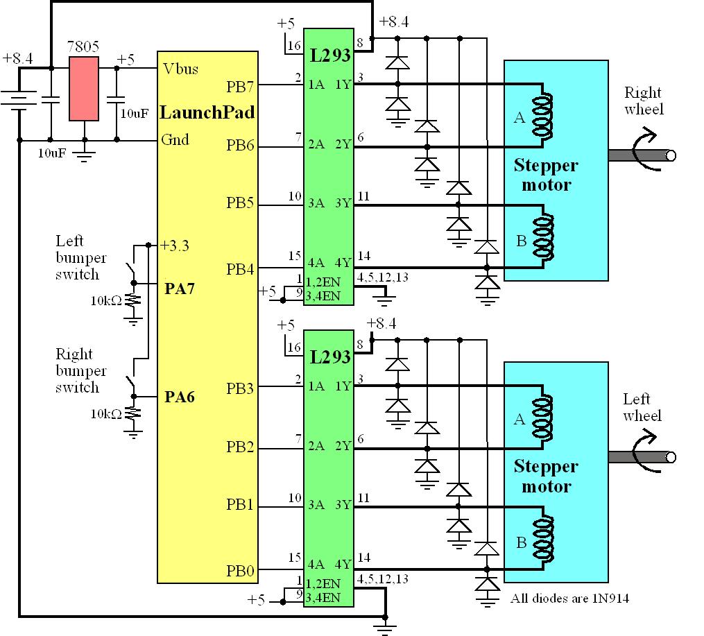
Figure 10.3.1. Two bipolar stepper motors interfaced to a microcontroller allow the robot to move. The dark lines carry large currents. Bipolar stepper motors have 4 wires.

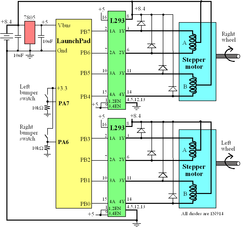
Figure 10.3.2. Two unipolar stepper motors interfaced to a microcontroller allow the robot to move. The dark lines carry large currents. Unipolar stepper motors have 5 or 6 wires.

To make the robot move forward (states 0,1,2,3) we spin both motors. To satisfy Isaac Asimov’s first law of robotics “A robot may not injure a human being or, through inaction, allow a human being to come to harm”, we will add two bumper switches in the front that will turn the robot if it detects an object in its path. To make the robot move backward (states S3, S2, S1, S0), we step both motors the other direction. We turn right by stepping the right motor back and the left motor forward (states S0, S7, S8, S9). We turn left by stepping the left motor back and the right motor forward (states S0, S4, S5, S6). Figure 10.3.3 shows the FSM to control this simple robot. This FSM has two inputs, so each state has four next states. Notice the 1-to-1 correspondence between the state graph in Figure 10.3.3 and the FSM[10] data structure in Program 10.3.2.

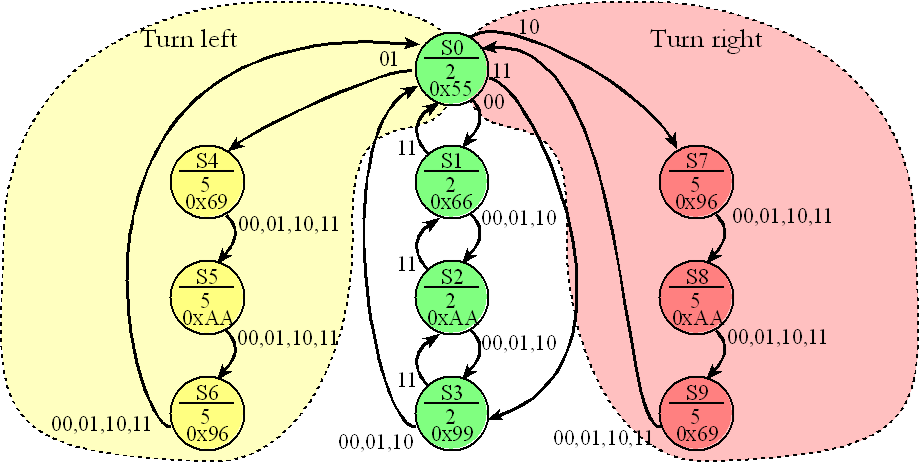
Figure 10.3.3. If the bumpers are not active (00) the both motor spin at 15 RPM, if both bumpers are active the robot backs up, if just the right bumper is active it turns left, and if just the left bumper is active, it turns right.

Program 10.3.1 shows the low-level code to perform input/output. Both implementations interface the two stepper motors to PB7-PB0. The TM4C123 system has the bump sensors connected to PE1-PE0, and the MSPM0 system connects the bumper switches to PA7-PA6. Using a board support package like this makes it easier to port the solution to other microcontrollers and other pins.

// TM4C123

void Robot_Init(void){

volatile uint32_t delay;

PLL_Init(Bus80MHz);

SYSCTL_RCGCGPIO_R |= 0x12;

delay = SYSCTL_RCGCGPIO_R;

GPIO_PORTB_PCTL_R = 0x00;

GPIO_PORTB_DIR_R = 0xFF;

GPIO_PORTB_AFSEL_R = 0x00;

GPIO_PORTB_DR8R_R = 0xfF;

GPIO_PORTB_DEN_R = 0xFF;

GPIO_PORTE_PCTL_R &= ~0xFF;

GPIO_PORTE_DIR_R &= ~0x03;

GPIO_PORTE_AFSEL_R &= ~0x03;

GPIO_PORTE_DEN_R |= 0x03;

}

void Robot_Output(uint32_t data){

GPIO_PORTB_DATA_R = data;

}

uint32_t Robot_Input(void){

return (GPIO_PORTE_DATA_R&0x03);

}

// MSPM0G3507

void Robot_Init(void){

Clock_Init80MHz(0);

LaunchPad_Init();

IOMUX->SECCFG.PINCM[PA7INDEX] = 0x00040081;

IOMUX->SECCFG.PINCM[PA6INDEX] = 0x00040081;

IOMUX->SECCFG.PINCM[PB7INDEX] = 0x00000081;

IOMUX->SECCFG.PINCM[PB6INDEX] = 0x00000081;

IOMUX->SECCFG.PINCM[PB5INDEX] = 0x00000081;

IOMUX->SECCFG.PINCM[PB4INDEX] = 0x00000081;

IOMUX->SECCFG.PINCM[PB3INDEX] = 0x00000081;

IOMUX->SECCFG.PINCM[PB2INDEX] = 0x00000081;

IOMUX->SECCFG.PINCM[PB1INDEX] = 0x00000081;

IOMUX->SECCFG.PINCM[PB0INDEX] = 0x00000081;

GPIOB->DOE31_0 |= 0xFF;

}

void Robot_Output(uint32_t data){

GPIOB->DOUT31_0 =

(GPIOB->DOUT31_0&(~0xFF))|data;

}

uint32_t Robot_Input(void){

return (GPIOA->DIN31_0&0xC0)>>6;

}

Program 10.3.1. Low-level software for the stepper motor robot.

The main program, Program 10.3.2, begins by initializing all of Ports B to be an output and PA1,PA0 to be an input. There are ten states in this robot. If the bumper switch activates, it attempts to turn away from the object. Every 20 ms the program outputs a new stepper commands to both motors. The function SysTick_Wait10ms()generates an appropriate delay between outputs to the stepper. For a 200 step/rotation stepper, if we wait 20 ms between outputs, there will be 50 outputs/sec, or 3000 outputs/min, causing the stepper motor to spin at 15 RPM. When calculating speed, it is important to keep track of the units.

Speed = (1 rotation/200 steps)*(1000ms/s)*(60sec/min)*(1step/20ms) = 15 RPM

Video 4.5.3. Robot Car - Software

Video 4.5.4. Robot Car - Demo

// represents a State of the FSM

struct State{

uint8_t out; // PB7-4 to right motor, PB3-0 to left

uint16_t wait; // in 10ms units

uint8_t next[4]; // input 0x00 means ok,

// 0x01 means right side bumped something,

// 0x02 means left side bumped something,

// 0x03 means head-on collision (both sides bumped something)

};

typedef const struct State State_t;

State_t Fsm[10] = {

{0x55, 2, {1, 4, 7, 3} }, // S0) initial state and state where bumpers are checked

{0x66, 2, {2, 2, 2, 0} }, // S1) both forward [1]

{0xAA, 2, {3, 3, 3, 1} }, // S2) both forward [2]

{0x99, 2, {0, 0, 0, 2} }, // S3) both forward [3]

{0x69, 5, {5, 5, 5, 5} }, // S4) left forward; right reverse [1] turn left

{0xAA, 5, {6, 6, 6, 6} }, // S5) left forward; right reverse [2] turn left

{0x96, 5, {0, 0, 0, 0} }, // S6) left forward; right reverse [3] turn left

{0x96, 5, {8, 8, 8, 8} }, // S7) left reverse; right forward [1] turn right

{0xAA, 5, {9, 9, 9, 9} }, // S8) left reverse; right forward [2] turn right

{0x69, 5, {0, 0, 0, 0} } // S9) left reverse; right forward [3] turn right

};

uint8_t cState; // current State (0 to 9)

int main(void){

uint8_t input;

SysTick_Init();

Robot_Init(); // initialize motor outputs on Port B, initialize sensor inputs on Port A

cState = 0; // initial state = 0

while(1){

// output based on current state

Robot_Output(Fsm[cState].out); // step motor

// wait for time according to state

SysTick_Wait10ms(Fsm[cState].wait);

// get input

input = Robot_Input(); // Input 0,1,2,3

// change the state based on input and current state

cState = Fsm[cState].next[input];

}

Program 10.3.2. Stepper motor controller.

10.4. Buddy Follower Robot using Fuzzy Logic

Example 10.4. Write RSLK robot software to follow you.

Solution: The RSLK robot has three Sharp GP2Y0A21YK0F or GP2Y0A41SK0F optical distance sensors as illustrated in Figure 10.4.1. The angles are 45° to left, center and 45° degrees to the right. The angles were selected so the three sensors have no blind spots. They are positioned away from the edge to eliminate the blind spot (non-monotonic behavior).

Figure 10.4.1. Three IR distance sensors on the RSLK robot.

The analog circuit is shown in Figure 10.4.2. Each sensor has a 10 uF capacitor on the Vcc to improve SNR. The analog outputs from the sensors are connected to analog inputs on the microcontroller. The maximum range of the GP2Y0A21YK0F is 800 mm, while the maximum range of the GP2Y0A41SK0F is 300 mm. The ADC produces a digital output dependent on its analog input. The Convert function calculates distance

   int32_t Convert(int32_t n){
     return A/(n+B);
   }

where A and B are calibration coefficients, n is the 12-bit sample, and return parameter is distance in mm. For details of this sensor see Section 2.3.1. ADC Parameters.

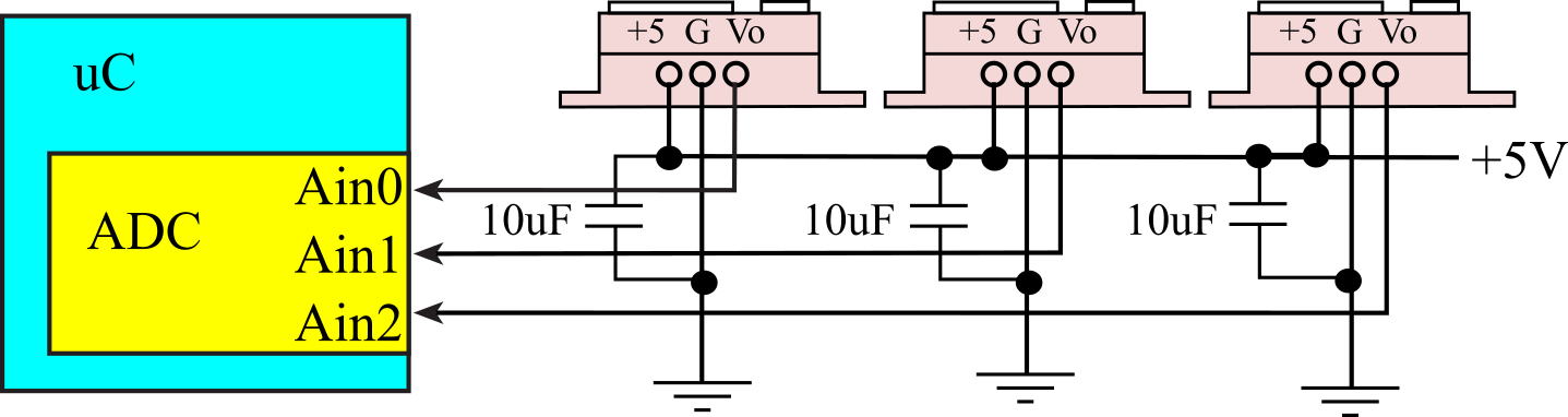
Figure 10.4.2. IR distance sensors on the RSLK robot. The interface uses three ADC channels.

Program 10.4.1 shows the high-level software using fuzzy logic to make the robot follow a safe distance behind you. Stage 1 implements the crisp inputs. Stage 2 implements the fuzzification, calculating the input membership sets. Stage 3 calculates the output membership sets using fuzzy logic. Stage 4 implements defuzzification creating the crisp outputs. The controller runs in the background using SysTick interrupts at 100 Hz. The robot will stop if one of the bump sensors is triggered.

// Fuzzy logic buddy follower

// Stage 1) Take measurements to determine crisp Inputs

int32_t Left; // distance to left object in mm

int32_t Center; // distance to center object in mm

int32_t Right; // distance to right object in mm

int32_t Distance; // distance to closed object in mm

int32_t LeftBuddy; // Center-Left, positive if closer to left

int32_t RightBuddy; // Center-Right, positive if closer to right

#define OVERFLOW 600 // over this value is no object

#define TURN 100

void Measurements(void){

Left = umin32(Convert(ADC_In(0)),OVERFLOW); // convert to signed

Center = umin32(Convert(ADC_In(1)),OVERFLOW); // convert to signed

Right = umin32(Convert(ADC_In(2)),OVERFLOW); // convert to signed

if(Bump_Read()){

Distance = 0; // crash

RightBuddy = 0;

LeftBuddy = 0;

}else{

Distance = min32(Left,Center,Right); // closest object

if(Right < Left){

LeftBuddy = 0;

if(Right < OVERFLOW){

if(Center < OVERFLOW){

RightBuddy = Center-Right;

}else{

RightBuddy = TURN;

}

}else{

RightBuddy = 0;

}

}else{

RightBuddy = 0;

if(Left < OVERFLOW){

if(Center < OVERFLOW){

LeftBuddy = Center-Left;

}else{

LeftBuddy = TURN;

}

}else{

LeftBuddy = 0;

}

// Stage 2) Determine Fuzzy Input Membership Set

#define TOOCLOSE 100 // minimum distance in mm

#define DESIRED 250 // desired distance in mm

#define TOOFAR 400 // max distance in mm

#define TOLERANCE 25 // +/- error is acceptable

#define MAXRANGE1 500 // out of range distance in mm

#define MAXRANGE2 600 // out of range distance in mm

fuz_t BuddyTooClose, OK, BuddyTooFar, NoBuddy; // distance sets

fuz_t BuddyToTheLeft,BuddyToTheRight; // turn sets

#define fs 100 // controller speed

void Fuzzification(void){

BuddyTooClose = MinFuzzification(Distance,TOOCLOSE,DESIRED-TOLERANCE);

OK = CenterFuzzification(Distance,TOOCLOSE,DESIRED,TOOFAR);

BuddyTooFar = MaxFuzzification(Distance,DESIRED+TOLERANCE,TOOFAR);

NoBuddy = MaxFuzzification(Distance,MAXRANGE1,MAXRANGE2);

BuddyToTheLeft = MaxFuzzification(LeftBuddy,0,TURN);

BuddyToTheRight = MaxFuzzification(RightBuddy,0,TURN);

}

// Stage 3) Determine Fuzzy Output Membership Set

fuz_t Forward,Hover,Backward,TurnLeft,GoStraight,TurnRight,Stop;

// Fuzzy logic converts input set to output set

void FuzzyLogic(void){

Stop = NoBuddy;

Hover = OK;

Backward = and(BuddyTooClose,not(NoBuddy));

Forward = and(BuddyTooFar,not(NoBuddy));

TurnLeft = and(BuddyToTheLeft,not(BuddyToTheRight));

GoStraight = and(not(BuddyToTheLeft),not(BuddyToTheRight));

TurnRight = and(not(BuddyToTheLeft),BuddyToTheRight);

}

// Stage 4) Transform output membership set to crisp Outputs

int32_t Power,Direction;

int32_t UR, UL; // PWM duty 0 to 14,998

int32_t Mode;

uint8_t Last;

#define MINDUTY 200

#define MAXDUTY 4000

#define GAIN 3000

#define STEERING 1500

void CheckDuty(void){

if(UR < MINDUTY) UR = MINDUTY;

if(UR > MAXDUTY) UR = MAXDUTY;

if(UL < MINDUTY) UL = MINDUTY;

if(UL > MAXDUTY) UL = MAXDUTY;

}

void Defuzzification(void){

if(NoBuddy >128){

Motor_Stop();

}else{

Power = (GAIN*(Forward-Backward))/(Forward+Hover+Backward);

Direction =(STEERING*(TurnLeft-TurnRight))/(TurnLeft+GoStraight+TurnRight);

if(Power > MINDUTY){

UR = UL = Power;

UR = UR + Direction;

UL = UL - Direction;

CheckDuty();

Motor_Forward(UL,UR);

Mode = 2; // forward

}else if (Power < -MINDUTY){

UR = UL = -Power;

UR = UR - Direction;

UL = UL + Direction;

CheckDuty();

Motor_Backward(UL,UR);

Mode = 3; // backward

}else{

if(Direction < -MINDUTY){

Mode = 4; // right

Motor_Right(-Direction,-Direction);

}else if(Direction > MINDUTY){

Mode = 5; // left

Motor_Left(Direction,Direction);

}else{

Motor_Stop();

Mode = 1;

}

void SysTick_Handler(void){

uint8_t in;

in = Bump_Read();

if(in&&(Last==0)){

Mode = 0; // stop

Distance = 0;

Motor_Stop();

}

Last = in;

if(Mode){

Measurements(); // Calculate distances to objects

Fuzzification(); // Sets input membership sets

FuzzyLogic(); // Sets output membership sets

Defuzzification(); // Calculate crisp output, set power to motors

}

int main(void){

Mode = 0; // stopped

Bump_Init(); // front bump switchs

Motor_Init(); // PWM outputs to left and right motors

ADC_Init(); // three ADC inputs from sensors

SysTick_Init(); // 100 Hz interrupt

while(1){

if(Mode == 0){ // stopped?

do{ // wait for touch

Clock_Delay10ms(30);

in = Bump_Read();

}while (in == 0);

while(Bump_Read()){ // wait for release

Clock_Delay10ms(150);

}

Mode = 1; // start

}

Program 10.4.1. High-level software to implement buddy following

Program 10.4.2 shows the low-level fuzzy logic functions.

typedef uint8_t fuz_t;

// Fuzzy NOT is complement

fuz_t not(fuz_t u1){

return 255-u1;

}

// Fuzzy AND is minimum

fuz_t and(fuz_t u1,fuz_t u2){

if(u1>u2){

return(u2);

}

return(u1);

}

// Fuzzy AND is minimum

fuz_t and3(fuz_t u1,fuz_t u2,fuz_t u3){

if(u1>u2){

if(u2>u3){

return u3;

}

return(u2);

}

if(u1>u3){

return u3;

}

return(u1);

}

// Fuzzy OR is maximum

fuz_t or(fuz_t u1,fuz_t u2){

if(u1<u2){

return(u2);

}

return(u1);

}

// Fuzzy OR is maximum

fuz_t or3(fuz_t u1,fuz_t u2,fuz_t u3){

if(u1<u2){

if(u2<u3){

return u3;

}

return(u2);

}

if(u1<u3){

return u3;

}

return(u1);

}

uint32_t umin32(uint32_t u1,uint32_t u2){

if(u1>u2){

return(u2);

}

else{

return(u1);

}

int32_t min32(int32_t n1,int32_t n2,int32_t n3){

if(n1>n2){

if(n2>n3){

return n3;

}

return(n2);

}

else{

if(n1>n3){

return n3;

}

return(n1);

}

fuz_t MinFuzzification(int32_t crisp, const int32_t MIN, const int32_t MAX){

if(crisp <= MIN){

return 255;

}

if(crisp >= MAX){

return 0;

}

return (255*(MAX-crisp))/(MAX-MIN);

}

fuz_t MaxFuzzification(int32_t crisp, const int32_t MIN, const int32_t MAX){

if(crisp <= MIN){

return 0;

}

if(crisp >= MAX){

return 255;

}

return (255*(crisp-MIN))/(MAX-MIN);

}

fuz_t CenterFuzzification(int32_t crisp, const int32_t MIN, const int32_t CENTER, const int32_t MAX){

if(crisp <= MIN){

return 0;

}

if(crisp >= MAX){

return 0;

}

if(crisp <= CENTER){

return (255*(crisp-MIN))/(CENTER-MIN);

}

return (255*(MAX-crisp))/(MAX-CENTER);

}

fuz_t LeftRightFuzzification(int32_t crisp, const int32_t MIN,

const int32_t LEFT, const int32_t RIGHT, const int32_t MAX){

if(crisp <= MIN){

return 0;

}

if(crisp >= MAX){

return 0;

}

if(crisp < LEFT){

return (255*(crisp-MIN))/(LEFT-MIN);

}

if(crisp > RIGHT){

return (255*(MAX-crisp))/(MAX-RIGHT);

}

return 255; // between LEFT and RIGHT

}

Program 10.4.2. Low-level software to implement fuzzy logic.

10.5. Autonomous Racing Robot using Performance Maps

Example 10.5. Write RSLK robot software that drives equidistance between two walls. Figure 10.5.1 shows a typical racetrack.

Figure 10.5.1. Austin GP Formula 1 racetrack. It can be built with 54 pieces of 4in by 4in by 3ft wood pieces.

Solution: We will use two TF-Luna distance sensors, one on each side of the robot. The angle to the wall should be adjusted to create reliable measurements. These optical sensors are based on the time-of-flight principle. It emits a modulated near IR wave periodically, which is reflected off the target. The round-trip time of flight is obtained by measuring the phase difference between transmitted and received wave, Δφ. Distance, D, is calculated knowing the frequency of the wave, f, and the speed of light, c. The interface is a full-duplex 8-bit no parity UART at 115200 bits/sec as shown in Figure 10.5.2. Although it is powered at +5V, the UART communication is 3.3V, so it can be directly connected to the TM4C123 or MSPM0.

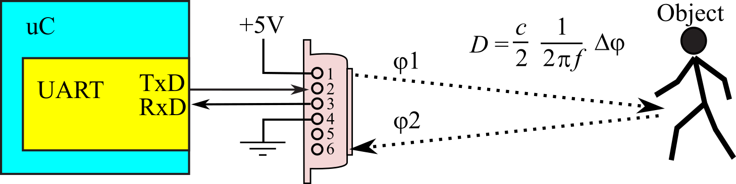
Figure 10.5.2. TF-Luna distance sensor.

The hardware interface uses UART. To initialize we send a sequence of commands strings. Each command starts with 0x5A, followed by a length, and ends in a checksum. Program 10.5.1 shows the minimum set of messages we send to the TF-Luna to configure operation. Command/status messages begin with 0x5A. The second frame is the message length, and the last frame is an 8-bit checksum.

const uint8_t Format_Standard_mm[5]={0x5A,0x05,0x05,0x06,0x6A};

#define TFLunaRate 100

#define SU1 ((0x5A+0x06+0x3+TFLunaRate)&0xFF)

const uint8_t Frame_Rate[6]={0x5A,0x06,0x03,TFLunaRate,0,SU1};

const uint8_t SaveSettings[4]={0x5A,0x04,0x11,0x6F};

const uint8_t System_Reset[4]={0x5A,0x04,0x02,0x60};

// expected response is 0x5A,0x05,0x02,0x00, 0x60 for success

// expected response is 0x5A,0x05,0x02,0x01, 0x61 for failed

Program 10.5.1. Messages needed to configure the TF-Luna.

After initialization, the TF-Luna will send 9-byte messages at 100 Hz with the distance in mm. If you use interrupts to receive these data messages, the software overhead for each TF-Luna is about 17µs every 10ms, or 0.17%.

{0x59,0x59,lowD,highD,lowStrength,highStrength,lowTemp,highTemp,chk}

For more information see data sheets

Benewake 10152020 TF-Luna Data Sheet

TF-Luna A01 Product Manual

The strategy for implementing the performance map begins with a finite number of fiduciary points using intuition. For example, what should we do if the robot is 250mm from both walls? Answer, "go normal speed and straight". This simple solution selects three distances, and like fuzzy logic, assigns meaning to each distance.

Close 100mm

Middle 250mm

Far 500mm

Since there are two sensors, there will be 9 scenarios as illustrated in Figure 10.5.3. Basically, the closer the robot is to a wall, the slower it will run. If it gets close to the left wall, it will turn right. If it gets close to the right wall it will turn left.

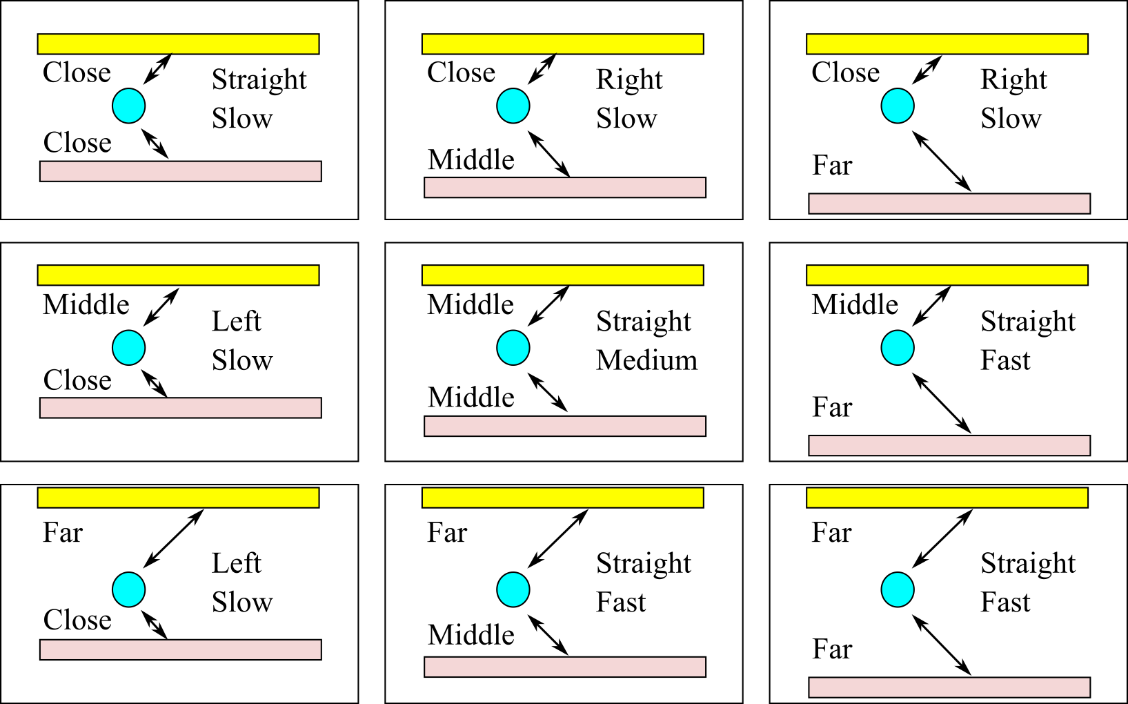
Figure 10.5.3. Intuition behind the performance map.

The performance map translates output states into actual motor commands

Left PWM Right PWM

Straight Slow 2000 2000

Right Slow 2250 1750

Left Slow 1750 2250

Straight Med 3000 3000

Straight Fast 5000 5000

Figure 10.5.4 shows the performance map for the right motor. The inputs are left and right distances, and the output is the right PWM. The map is defined by these nine points. However, using interpolation there is a unique output for all left and right distances from 100 to 500 mm.

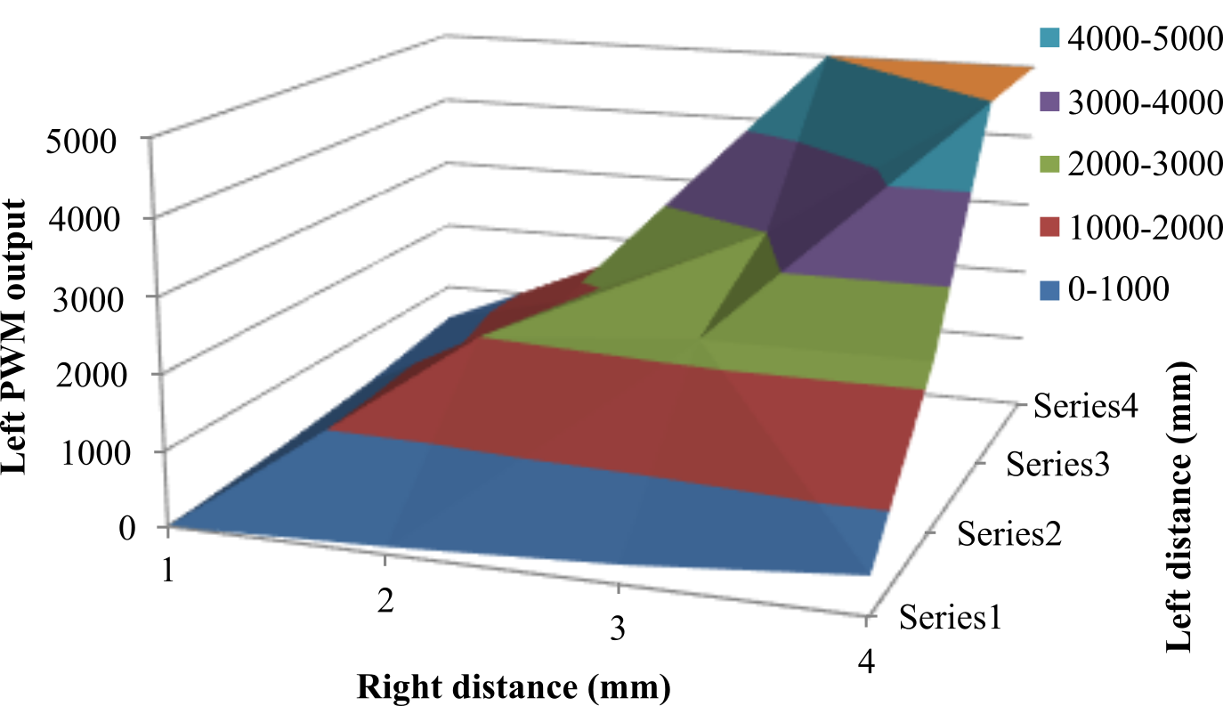
Figure 10.5.4. The performance map converts left and right distance into right PWM (there is a similarly formatted performance map for the left PWM).

Program 10.5.2 shows the data structures that define the two performance maps.

// Right distances 100 250 or 500 mm, I= 0, 1, 2
// Left distances 100 250 or 500 mm, J= 0, 1, 2
const int32_t RightMap[3][3]={ // PWM outputs
{2000, 1750, 1750},
{2250, 3000, 5000},
{2250, 5000, 5000}
};
const int32_t LeftMap[3][3]={ // PWM outputs
{2000, 2250, 2250},
{1750, 3000, 5000},
{1750, 5000, 5000}
};

Program 10.5.2. Performance map converts left and right distance into right and left PWMs.

Let x be the distance to the left wall in mm. Let y be the distance to the right wall in mm. First, we search performance map for x₁, x₂, y₁, and y₂ which for this map will be 100, 250 or 500 mm. https://en.wikipedia.org/wiki/Bilinear_interpolation

Given (x,y) find four points x₁≤ x ≤ x₂for y₁≤ y ≤ y₂
    Q₁₁ = (x₁, y₁), Q₁₂ = (x₁, y₂), Q₂₁ = (x₂, y₁), Q₂₂ = (x₂, y₂)
Weights
    w₁₁ = ((x₂- x)*(y₂- y))/((x₂- x₁)*(y₂- y₁))
    w₁₂ = ((x₂- x)*(y - y₁))/((x₂- x₁)*(y₂- y₁))
    w₂₁ = ((x - x₁)*(y₂-y))/((x₂- x₁)*(y₂- y₁))
    w₂₂ = ((x - x₁)*(y - y₁))/((x₂- x₁)*(y₂- y₁))
Interpolate
    leftPWM = w₁₁*LeftMap(Q₁₁) + w₁₂* LeftMap(Q₁₂) + w₂₁* LeftMap(Q₂₁) + w₂₂* LeftMap(Q₂₂)
   rightPWM = w₁₁*RightMap(Q₁₁) + w₁₂* RightMap(Q₁₂) + w₂₁* RightMap(Q₂₁) + w₂₂* RightMap(Q₂₂)

10.6. Lab 10. Final Design and Evaluation of an Embedded System

Lab 10 for this course can be downloaded from this link Lab10.docx

Each lab also has a report Lab10Report.docx and

This work is based on the course ECE445L taught at the University of Texas at Austin. This course was developed by Jonathan Valvano, Mark McDermott, and Bill Bard.

Reprinted with approval from Embedded Systems: Real-Time Interfacing to ARM Cortex-M Microcontrollers, ISBN-13: 978-1463590154

Embedded Systems: Real-Time Interfacing to ARM Cortex-M Microcontrollers by Jonathan Valvano is licensed under a Creative Commons Attribution-NonCommercial-NoDerivatives 4.0 International License.