8. Control Systems
Table of Contents:
- 8.1. Introduction to Digital Control Systems
- 8.2. Input Capture
- 8.2.1. Basic Principles
- 8.2.2. Measurement of Resistance
- 8.2.3. Optical Encoder
- 8.2.4. Tachometer to measure motor speed
- 8.2.5. Measurement of Capacitance
- 8.2.6. Line Sensor
- 8.3. Binary Actuators
- 8.3.1. Electrical Interfaces
- 8.3.2. Electromagnetic and Solid-State Relays
- 8.3.3. Solenoids
- 8.3.4. Brushed DC Motor
- 8.3.5. Robot Systems Learning Kit (RSLK2)
- 8.3.6. Brushless DC Motor (BLDC)
- 8.3.7. Stepper Motors
- 8.4. Pulse Width Modulation
- 8.5. Odometry
- 8.6. Simple Closed-Loop Control Systems
- 8.7. PID Controllers
- 8.7.1. General Approach to a PID Controller
- 8.7.2. Design Process for a PID Controller
- 8.7.3. PI Controller Example
- 8.7.4. PID Controller Example
- 8.8. Fuzzy Logic Control
- 8.9. Lab 8. RSLK Motor Control
Chapter 8 objectives are to:
• Use input capture to measure period or pulse width or frequency
• Interface coil-activated devices like DC motors, solenoids, and relays
• Interface an optical tachometer
• Generate waveforms using the pulse-width modulator
• Design and implement a control system
The timer systems on state-of-the-art microcontrollers are very versatile. This chapter introduces fundamental principles of time used as an input and as an output. Over the last 40 years, the evolution of these timer functions has paralleled the growth of new applications possible with these embedded computers. In other words, inexpensive yet powerful embedded systems have been made possible by the capabilities of the timer system. To measure motor speed, we will use a tachometer an employ the timer in input capture mode to measure period. To adjust power to a DC motor, we will use a time-based method called pulse-width modulation. To control the rotational speed of the motor, we combine tachometer input and PWM output, and we write a closed loop controller in software, see Figure 8.1.1.
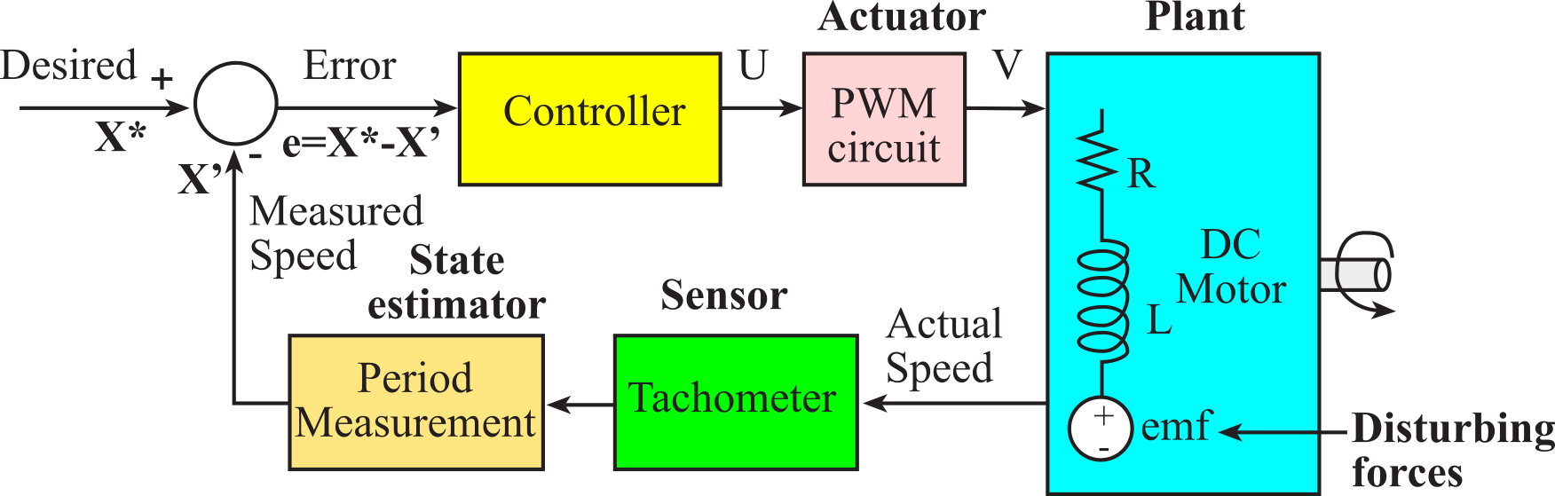
Figure 8.1.1. Block diagram of a microcomputer-based closed-loop control system.
A control system is a collection of mechanical and electrical devices connected for the purpose of commanding, directing, or regulating a physical plant. The real state variables are the properties of the physical plant that are to be controlled. The sensor and state estimator comprise a data acquisition system. The goal of this data acquisition system is to estimate the state variables. A closed-loop control system uses the output of the state estimator in a feedback loop to drive the errors to zero. The control system compares these estimated state variables, X'(t), to the desired state variables, X*(t), to decide appropriate action, U(t). The actuator is a transducer that converts the control system commands, U(t), into driving forces, V(t), that are applied to the physical plant. In general, the goal of the control system is to drive the real state variables to equal the desired state variables. It is important to have an accurate state estimator, because any differences between the estimated state variables and the real state variables will translate directly into controller errors. If we define the error as the difference between the desired and estimated state variables:
e(t) = X*(t)- X'(t)
then the control system will attempt to drive e(t) to zero. In general control theory, X(t), X'(t), X*(t), U(t), V(t) and e(t) refer to vectors, but the examples in this chapter control only a single parameter. Even though this chapter shows one-dimensional systems, and it should be straight-forward to apply standard multivariate control theory to more complex problems. We usually evaluate the effectiveness of a control system by determining three properties: steady state controller error, stability, and transient response.
An open-loop control system does not include a state estimator. It is called open loop because there is no feedback path providing information about the state variable to the controller. It will be difficult to use open loop with the plant that is complex because the disturbing forces will have a significant effect on controller error. On the other hand, if the plant is well-defined and the disturbing forces have little effect, then an open-loop approach may be feasible. Because an open-loop control system does not know the current values of the state variables, large errors can occur. Stepper motors are often used in open loop fashion.
Observation: You cannot control anything you cannot measure.
The steady state controller error is the average value of e(t)=|Desired-Actual|. Because load on the physical plant (e.g., friction) will affect performance, it is important to measure error under load conditions typical of how the controller will be used.
: Consider a control system with an average error of +10 rps error in its state estimator, what is the expected error in the control system?
Stability means the controller will eventually settle at a constant speed, given constant load and constant desired speed. A system with small and transient oscillations is stable. An unstable system oscillates, or it may saturate. The error is small and bounded on a stable system.
The transient response is defined as the time to new steady state after a change in desired or a change in load, see Figure 8.1.2. More specifically is how long the system takes to reach 99% of the final output after X* is changed. A system is stable if steady state (smooth constant output) is achieved.
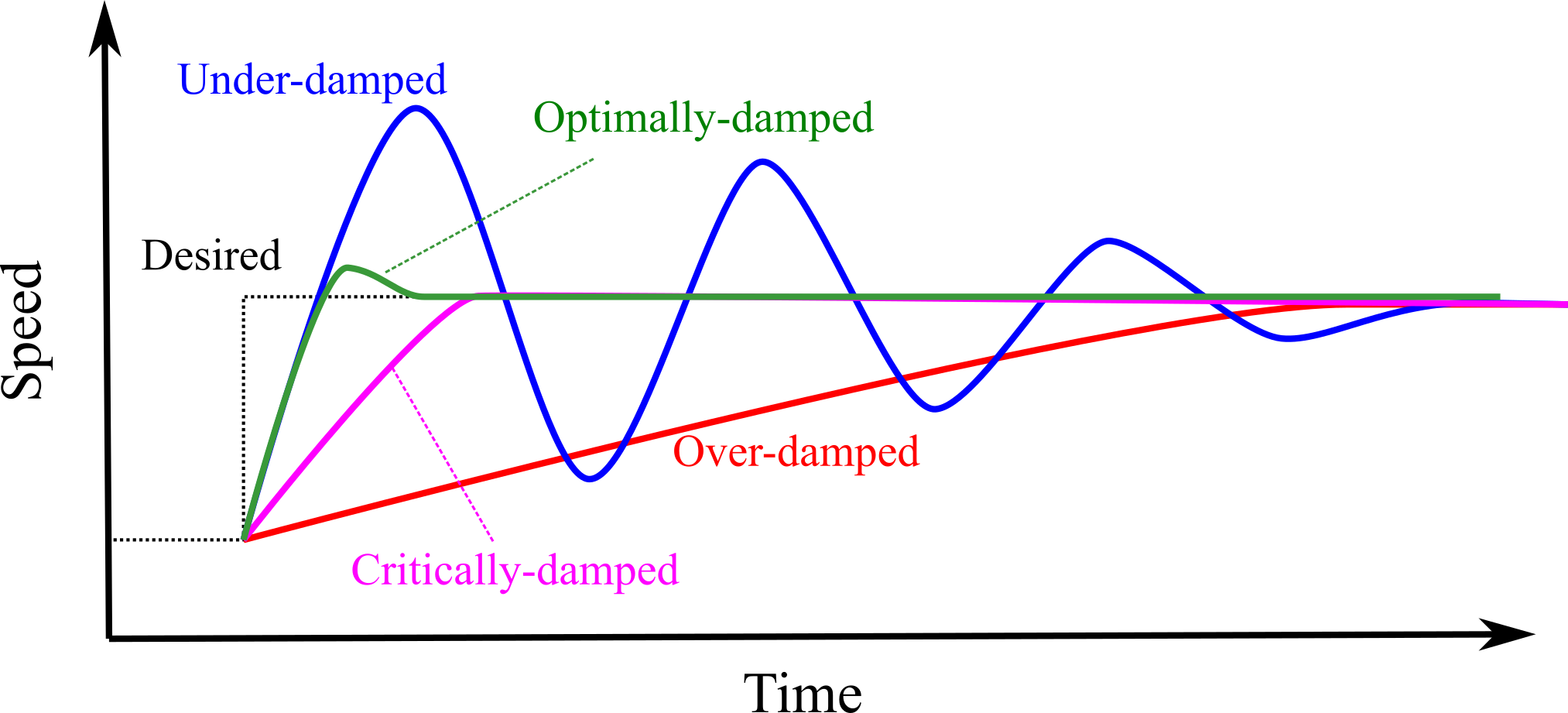
Figure 8.1.2. Response time for a controller.
An under-damped system has some ringing, which we will still classify as stable if the ringing is small and short. We can sometimes remove underdamping by decreasing the control constants Ki and Kp. When tuning a controller, it is best to change one constant at a time.
A critically-damped system has a response time similar to the time constant of the motor and has no overshoots.
An optimally-damped system has a response time shorter than critically damped with some overshoots.
An over-damped system has a very long response time compared to the time constant of the motor. We can sometimes remove overdamping by increasing the control constants Ki and Kp.
8.2.1. Basic Principles
We will use input capture to measure period, pulse width, duty cycle or frequency. The basic idea is to connect a digital signal to an input capture pin. There is a free running n-bit counter. The hardware decrements the counter at a fixed rate derived from the bus clock. The time measurement will be accurate because of the stability of the crystal. A capture event stores the n-bit counter value into the n-bit latch register, as shown in Figure 8.2.1. We can capture on a rising edge, falling edge, or both edges. The capture event also sets a hardware flag, which can generate an interrupt.
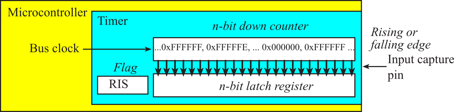
Figure 8.2.1. Input capture using a counter, a latch, and an interrupt flag.
Period, P, is defined as the time from rising edge to the next rising edge, as shown in Figure 8.1.2. We could measure the period from falling edge to the next falling edge.

Figure 8.2.2. Period is the time from rising edge to rising edge.
To measure the period, we connect the input signal to a capture pin. On the rising edge of the capture pin, the hardware stores the counter into the latch. The capture event will also set a hardware flag, and that flag will trigger an interrupt. There are static variables, Last and Now, containing the previous and current latched values. To measure the period, the ISR performs
1. Set variable Now to the value of the n-bit latch register
2. Calculate Period = Last-Now, as an n-bit subtraction
3. Set Last = Now, getting ready for the next interrupt
When measuring period, the measurement resolution will equal the period of the clock decrementing the counter. The precision will be the number of bits in the counter. Assuming a 24-bit latch value, the following C code performs a 24-bit subtraction.
Period = (Last-Now)&0x00FFFFFF;
: When does an input capture event occur?
: What happens during an input capture event?
: What is the range, resolution, and precision of a period measurement using a 16-bit counter clocked at 16 MHz?
Pulse width, PW, is the time from a rising edge to the next falling edge, as shown in Figure 8.2.3.

Figure 8.2.3. Pulse width is the time from a rising edge to the next falling edge.
To measure pulse width, we capture on both edges. When measuring pulse-width, the measurement resolution will equal the period of the clock decrementing the counter. The precision will be the number of bits in the counter. The capture events will set a hardware flag, and that flag will trigger an interrupt. There are two static variables, Rise and Fall. To measure pulse width, the ISR performs
1. If this is rising edge, set variable Rise to the value of the n-bit latch register
2. Else (if this is falling edge)
a) set variable Fall to the value of the n-bit latch register
b) PW = Rise-Fall, as an n-bit subtraction
: How do you measure the duty cycle of an input signal?
The direct measurement of frequency involves counting input pulses for a fixed amount of time. The basic idea is to use input capture to count pulses and use a periodic interrupt to create the fixed-time interval, Δt, as shown in Figure 8.2.4.
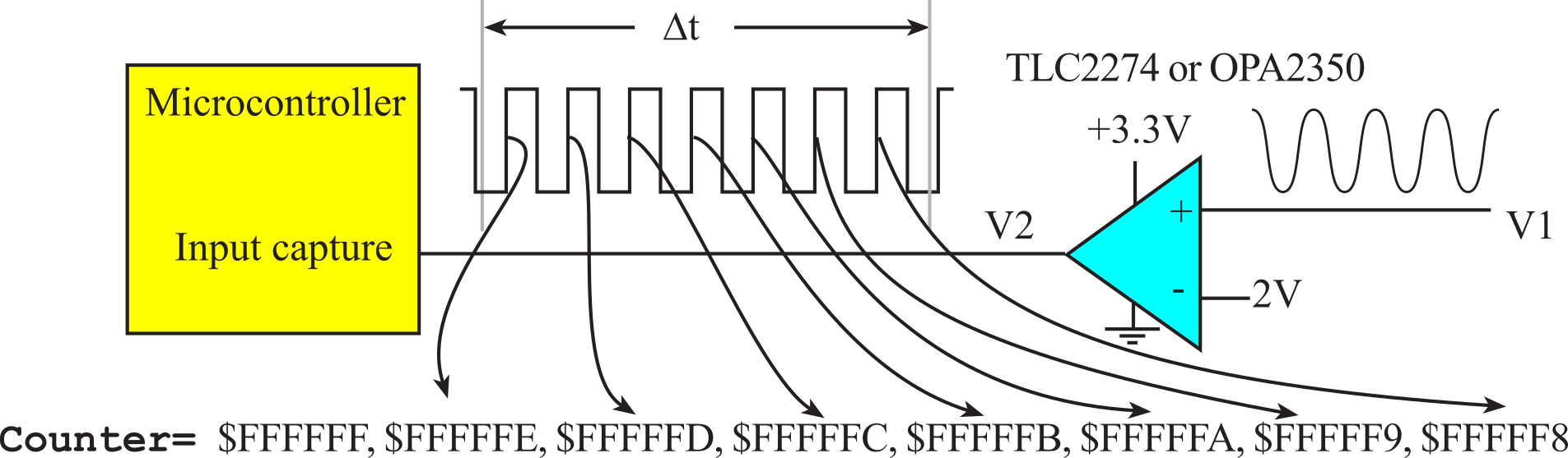
Figure 8.2.4. Frequency is the number of pulses occurring in a fixed-time interval, Δt.
We could initialize input capture to decrement a Counter on every rising edge of our input signal. The reload value for the Counter is set to its maximum, max. We create a periodic interrupt at Δt. During the periodic interrupt, we perform:
1. Calculate Frequency = max-Counter; with units of 1/Δt
2. Reload the Counter to its maximum, max
The frequency resolution, ∆f, is defined to be the smallest change in frequency that can be reliably measured by the system. For the system to detect a change, the frequency must increase (or decrease) enough so that there is one more (or one less) pulse during the fixed time interval. Therefore, the frequency resolution is
∆f = 1/Δt
This frequency resolution also specifies the units of the measurement. E.g., if Δt is 10ms, the frequency resolution is 100Hz. Let Δt be 10ms in Figure 8.2.4. max=0xFFFFFF, Counter is 0xFFFFF8 at the second ISR, and Frequency=7, meaning 700 Hz. See Appendix T.9.3 for implementation on the TM4C123.
: In frequency measurement, what happens on an input capture event?
Period and frequency are obviously related, so when faced with a problem that requires frequency information, we could measure period and calculate frequency from the period.
If we have a timer clock of 8 MHz, the period measurement system will have a resolution of 125 ns. Assume p is 16-bit period measurement. With a resolution of 125ns, the period can range from about 40 to 8192 µs. This corresponds to a frequency range of 122 Hz to 25 kHz. We can calculate frequency f from this period measurement, f = 8000000/p
It is easy to see how the 40 to 8192 µs period range maps into the 122 Hz to 25 kHz frequency range, but mapping the 125 ns period resolution into an equivalent frequency resolution is a little trickier. If the frequency is f, then the frequency must change to f+∆f such that the period changes by at least ∆p= 125 ns. 1/f is the initial period, and 1/(f+∆f) is the new period. These two periods differ by 125 ns. In other words,
![]()
We can rearrange this equation to relate ∆f as a function of ∆p and f.
![]()
This very nonlinear relationship, shown in Table 8.2.1, illustrates that although the period resolution is fixed at 125 ns, the equivalent frequency resolution varies from 500 Hz to 0.0005 Hz. If we restrict the signal frequency to the range from 125 to 2828 Hz, then we can say the frequency resolution will be better than 1 Hz.
|
Frequency (Hz) |
Period (µsec) |
∆f (Hz) |
|
25000 |
40 |
78.370 |
|
16000 |
63 |
32.064 |
|
8000 |
125 |
8.008 |
|
2000 |
500 |
0.500 |
|
1000 |
1000 |
0.125 |
|
500 |
2000 |
0.031 |
|
250 |
4000 |
0.008 |
|
125 |
8000 |
0.002 |
Table 8.2.1. Relationship between frequency resolution and frequency when calculated using period measurement.
Similarly, when faced with a problem that requires a period measurement, we could measure frequency and calculate period from the frequency measurement. A similar nonlinear relationship exists between the frequency resolution and period resolution. In general, the period measurement approach will be faster, but the frequency measurement approach will be more robust in the face of missed edges or extra pulses.
![]()
8.2.2. Measurement of Resistance
We will design a system to measure resistance and use it to interface a 10-kΩ joystick. You could just connect the potentiometer across the power rails and measure the voltage drop using the ADC. However, it is much cheaper and easier to measure time precisely than to measure voltage precisely. This makes sense, considering that an inexpensive clock can run for months before it needs to be reset, but even a high-quality voltmeter requires frequent calibration. Therefore, we will convert the resistance to a pulse width using external circuitry and measure the pulse using input capture. If the timer runs at 80 MHz, the pulse width resolution will be 12.5 ns. If we use a 24-bit timer, the range will be 10 µs to 209 ms. With the minimum determined by the time to execute software and the maximum determined by the 24-bit counter (12.5 ns *224.) The desired resistance measurement range is 0 to 10 kΩ, the desired resolution is 1 Ω.
Figure 8.2.5. To measure resistance using pulse width we connect the external signal to two input capture pins.
Most joysticks have two variable resistances, but we will show the solution for just one of the potentiometers. The variable resistance R in Figure 8.2.5 is one channel of the joystick. We use a monostable to convert unknown resistance, R, to time difference t. To perform high quality measurements, we will need a high-quality capacitor, because of the basic conversion follows Δt = R*C. We connect a PWM output to B and connect two input capture pins to Q. A rising edge on B causes a monostable positive logic pulse on the "Q" output of the 74HC123. The first input capture measures the time of the rising edge. The second input capture measures the time of the falling edge. The pulse width, t, is the difference between the two captures.
We choose R1 and C, so that the resistance resolution maps into a pulse width measurement resolution of 12.5 ns, and the resistance range 0 ≤ R ≤ 10 kΩ maps into 125 ≤ t ≤ 250 µs. The following equation describes the pulse width generated by the 74HC123 monostable as a function of resistance and capacitance.
t = 0.45* (R +R1) *C
For a linear system, with x as input and y as output, we can use calculus to relate the measurement resolution of the input and output.
![]()
Therefore, the relationship between the pulse width measurement resolution, ∆t, and the resulting resistance measurement resolution is determined by the value of the capacitor.
Δt = 0.45 * ΔR * C
To make a ∆t of 12.5 ns correspond to a ΔR of 1 Ω, we choose
C=∆t/(0.45ΔR)=12.5ns/(0.45*1Ω)=27.8nF
We will use a C0G high-stability 27nF ceramic capacitor. To design for the minimum pulse width, we set R=0, t=0.45*R1*C. We choose R1 to make the minimum pulse width 125 µs,
R1=t/(0.45*C)=125µs/(0.45•27nF) = 10.288 kΩ
We will use a 1% metal film 10-kΩ resistor for R1. To check the minimum and maximum pulse widths we set R=0 and R1=10kΩ, and calculate t= 0.45*(10kΩ)*27nF=121.5µs (close to 125), and t= 0.45* (20kΩ) *27nF=243µs (close to 250). The parameters R1 and C are selected for their long-term stability. I.e., their performance should be constant over time. Any differences between assumed values and real values for the capacitor and the 0.45 constant can be compensated for with software calibration. The initialization software performs
Enable the PWM output to create a 1 kHz wave at B
Enable the first input capture to capture on rising edges without interrupts
Enable the second input capture to capture on falling edges with interrupts
Each invocation of the second input capture ISR calculates the resistance, R, in Ω. For example, if the resistance, R, is 1234 Ω, then R will be 1234. We will not worry about resistances, R, greater than 55535 Ω or if R is disconnected. There are two static variables, Rise and Fall. The second input capture ISR performs:
Set Rise variable to the value of the first n-bit latch register
Set Fall variable to the value of the second n-bit latch register
Calculate PW = Rise-Fall, as an n-bit subtraction
Calculate R =m* PW + b, where m and b are calibration coefficients
8.2.3. Optical Encoder
We will design a measurement system that counts the number of wheel rotations. See Section 8.5 on how to odometry to convert rotations into robot position. This count will be a measure of the total distance travelled. The desired resolution is 1/32 of a turn. Whenever you measure something, it is important to consider the resolution and range. The basic idea is to use an optical sensor (QRB1134) to visualize the position of the wheel. We attach a black/white striped pattern to the wheel and an optical reflective sensor near the stripes, see Figure 8.2.6. The sensor has an infrared LED output and a light sensitive transistor. The resolution will be determined by the number of stripes and the ability of the sensor to distinguish one stripe from another. The range will be determined by the precision of the software global variable used to count edges.
Figure 8.2.6. We use input capture to measure the number of rotations of a wheel.
The basic idea is to trigger an interrupt on each stripe and then count the stripes in the interrupt service routine (Count++). If there are 32 stripes on the pattern, then the number of times the wheel has turned will be Count/32. We can consider the variable Count as the integer part of a binary fixed-point number with a resolution of 2-5 revolutions. E.g., if the Count is 100, this means 100/32 or 3.125 revolutions. If the circumference of the wheel is fixed, and if the wheel does not slip, then this count is also a measure of distance traveled.
The current from anode to cathode controls the amount of emitted IR light. The operating point for the LED in the QRB1134 is 15 mA at 1.8 V. The R1 resistor sets the current to the LED. In this circuit, the LED current will be (3.3-1.8V)/R1, which we set to 15 mA by making R1 equal to 100Ω. The R2 pull-up resistor on the transistor creates an output swing at V1 depending on whether the sensor sees a black stripe or white stripe. Unfortunately, the signal V1 is not digital. The rail-to-rail op amp, in open loop mode, creates a clean digital signal at V2, which has the same frequency as V1. The negative terminal is set to a voltage in the center of V1, shown as +2V in Figure 8.2.6. Slew rate is defined as dV/dt. An uncertainty in voltage δV will translate to an uncertainty in time, δt = δV /(dV/dt). Thus, to minimize time error, we choose a place with maximum slew rate. In other words, we should select the threshold at the place in the wave where the slope is at maximum.
We then interface V2 to an input capture pin, and we configure the system to trigger an interrupt on each rising edge. Figure 8.2.7 shows scope tracings of V1 and V2. You can find a TM4C123 solution in Appendix T.9.3.
Figure 8.2.7. Measured V1 and V2 from the circuit in Figure 8.2.5.
: Derive an equation between Count and distance travelled.
8.2.4. Tachometer to measure motor speed
A Hall Effect Sensor is a simple and reliable way to measure motor shaft speed. Figure 8.2.8 shows permanent magnets are moving on the shaft and the sensor is stationary.
Figure 8.2.8. Magnets rotate on the shaft and the sensor is positioned near the magnets ( http://simplemotor.com/hall-effect-motor/).
Figure 8.2.9. shows how the permanent magnets on the shaft affect the sensor. The sensor outputs highs and lows as the motor spins. For the Pololu item #3675 the frequency of the sensor output is 360 times the wheel speed in rps, which combines the number of magnets times the gear ratio in the motor.
Figure 8.2.9. The Hall Effect Sensor detects the presence or absence of a magnetic field. ( http://www.electronics-tutorials.ws/electromagnetism/hall-effect.html).
We design a system that measures the rotational speed of two motors using period measurement with a precision of n=24 bits and a resolution of Δt =12.5 ns. The Robot Systems Learning Kit has Hall effect sensors on ELA and ERA, see Figures 8.2.10 and 8.2.11. In this example, we will measure the speed of both motors using two input captures. Each sensor has two outputs, A and B, which are 90 degrees out of phase. We could use B to determine the direction of rotation, but in this example the B signal will not be connected (just the two A signals). Let N=360 be the number of rising edges as the wheel rotates once. We will make the bus clock equals 80 MHz, resulting in a period resolution of Δt = 12.5ns. Each rising edge will generate an input capture interrupt.
Figure 8.2.10. To measure motor speed, we connect the tachometer signals to input capture pins.
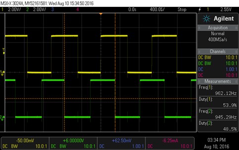
Figure 8.2.11. If the tach frequency is 962 Hz, then the wheel is spinning at 962/360 rps.
The left and right measurements are independent, meaning we measure them separately. The period is calculated as the difference in latch values from one rising edge to the next rising edge. Let Speed have units of RPM. If N=360, and the motor is spinning at 83.3 RPM, then the Period in ms will be
Period (ms) = [(60000ms/min)/(Speed RPM)/N edges/rotation)],
which will be 2.00 ms/edge. With Δt = 12.5ns, the 2ms creates an n-bit difference between latch values of 160,000. This subtraction remains valid even if the timer reaches zero and wraps around in between interrupts. On the other hand, this method will not operate properly if the period is larger than 2n cycles, or about 209 ms for n=24. 209 ms corresponds to a rotational speed of about 1 RPM. We will use a 100ms periodic interrupt to detect a motor spinning slower than 2 RPM.
Let Rot be the integer portion of a fixed-point number with units 0.1RPM. For example, if the speed is 83.3 RPM, Rot will be 833. Let Delta be the difference in latch values with units of 12.5ns clock cycles. For example, if the Period is 2 ms, Delta will be 160000.
Delta (cycles) = (80000 cycles/ms)[(60000ms/min)/(Speed RPM)/N edges/rotation)],
Delta (cycles) = 10*(80000cycles/ms)[(60000ms/min)/(Rot 0.1RPM)/N edges/rotation)],
Solving for Rot in terms of Delta
Rot 0.1RPM = 10*(80000cycles/ms)[(60000ms/min)/( Delta (cycles))/N edges/rotation)],
Rot = 133,333,333/Delta
The initialization software performs
Enable the first input capture to capture on rising edges on ELA with interrupts
Enable the second input capture to capture on rising edges on ERA with interrupts
Enable a periodic interrupt at 10Hz, 100ms
There are many static variables: LeftLast, LeftNow, LeftDelta, LeftRot, LeftCount, RightNow, RightDelta, RightRot, RightCount, and RightLast. The first input capture ISR calculates the speed of the left motor:
Set LeftNow variable to the value of the first n-bit latch register
Calculate LeftDelta = (LeftLast - LeftNow) as an n-bit subtraction
Calculate LeftRot = 133333333/LeftDelta with units of 0.1 RPM
LeftLast = LeftNow setup for next
LeftCount++
The second input capture ISR calculates the speed of the right motor:
Set RightNow variable to the value of the second n-bit latch register
Calculate RightDelta = (RightLast - RightNow) as an n-bit subtraction
Calculate RightRot = 133333333/RightDelta with units of 0.1 RPM
RightLast = RightNow setup for next
RightCount++
The 10 Hz periodic ISR detects if either or both motors are stopped:
If LeftCount is less than 2, set LeftRot = 0
If RightCount is less than 2, set RightRot = 0
Set LeftCount = RightCount = 0
At 1 RPM, the count should be larger than 2. If the speed is less than 1 RPM, the count will be 0 or 1, and the periodic ISR sets the speed to 0.
: How does this system recognize a stopped motor if no input capture interrupts occur?
8.2.5. Measurement of Capacitance
An effective approach to measure capacitance is to convert the electrical parameter to time. The example in Section 8.2.2 could have been used to measure capacitance. However, this approach has accuracy limitations of the 74HC123 monostable. This next approach will be more accurate because accuracy will depend only on the resistor value and the input capture measurement.
Let R be the value of a precision resistor. We will use an RC circuit to convert the input capacitance (C) to a time pulse width (Δt). Figure 8.2.12 shows the hardware circuit and typical waveforms. The PWM output can be any digital periodic wave, with a period long enough for the measurement to complete with C at its maximum. The waveform V2 is
V2(t) = 3.3 - 3.3e-t/RC
Capacitance is determined by measuring the time difference between the two input captures, Δt. The time Δt at when V2=2V is linearly related to C.
2 = 3.3 - 3.3e-Δt/RC
e-Δt/RC = 1.3/3.3
e+Δt/RC = 3.3/1.3
Δt/RC = ln(3.3/1.3)
C = Δt /(R*ln(3.3/1.3))
The purpose of adding the buffer and threshold detector to the reference signal V1 is to make the difference between V1 and V3 be independent of the buffer and detector, and only dependent on R and C.
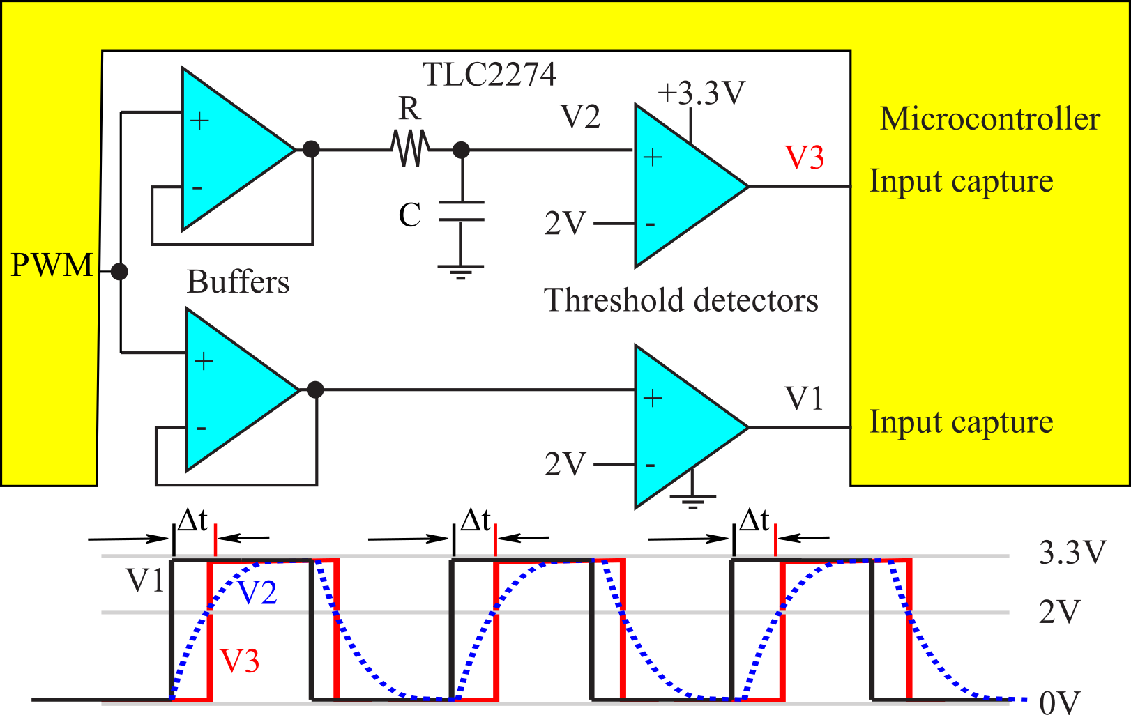
Figure 8.2.12. A capacitance meter uses two input capture pins.
The initialization software performs
Enable the PWM output to create a periodic square wave
Enable the first input capture to capture on rising edges on V1 without interrupts
Enable the second input capture to capture on rising edges on V3 with interrupts
Each invocation of the second input capture ISR calculates the capacitance, C. There are two static variables, Rise1 and Rise3. The second input capture ISR performs:
Set Rise1 variable to the value of the first n-bit latch register
Set Rise3 variable to the value of the second n-bit latch register
Calculate PW = Rise1-Rise3, as an n-bit subtraction
Calculate C =m* PW + b, where m and b are calibration coefficients
: What factors determine the resolution of the capacitance measurement?
8.2.6. Line Sensor
A line sensor can be placed on the bottom of a robot to detect the presence or absence of a line. Pololu makes a series of optical reflectance sensors having 1 to 16 measurements. Figure 8.2.13 shows a line sensor with 8 positions. The optimal sensing distance for the Pololu sensor is 10mm.
https://www.pololu.com/category/123/pololu-qtr-reflectance-sensors
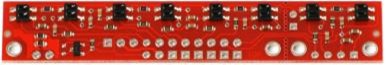
Figure 8.2.13. Pololu QTRX-8 sensor.
Figure 8.2.14 shows an interface circuit. There is one output, which is used to activate the IR LED. The other pin is first an output, then an input. The QTRX-8 has 8 sensors, so it has one signal to activate all 8 IR LEDs, and 8 separate Out/In signals, one for each sensor.
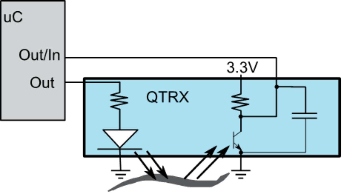
Figure 8.2.14. Pololu QTRX interface.
The measurement sequence is
1) Set Out high (turn on IR LED)
2) Make Out/In an output, and set it high (charging the capacitor)
3) Wait 10 us,
4) Make Out/In an input
5) Measure width with falling edge input capture
Figure 8.2.15 shows typical waveforms for reflective and absorbing surfaces. The 10us pulse charges the capacitor in the interface. If the surface is reflecting (left), the sensor conducts more current and the capacitor discharges quickly. If the surface is absorbing (right), the sensor conducts less current and the capacitor discharges more slowly. The yellow trace is the Out/In pin, and the blue trace is the corresponding value when the microcontroller reads the Out/In pin as a digital input.
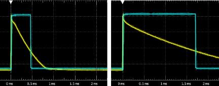
Figure 8.2.15. Pololu QTRX waveforms.
Rather than using input capture we could find a time (1ms) at which the absorbing surface reads high, and the reflecting surface reads low. This simple approach performs steps 1-4 above, waits 1ms, and then reads the Out/In pin as a digital input. Notice in Figure 8.2.15 at 1ms, the reflecting surface shows low and absorbing surface is high. To run the measurement in the background we will use two timer interrupts. The initialization is
Enable a periodic timer interrupt at desired sampling rate (greater than 10ms)
Configure a second timer, but do not arm it.
Enable the Out pin as an output low
Enable the Out/In pin as an input
The periodic ISR performs steps 1 to 4
1) Set Out high (turn on IR LEDs)
2) Make the Out/In pins output, and set them high (charging the capacitors)
3) Wait 10 us,
4) Make Out/In pins input
5) Arm the second timer to interrupt 1ms later
The second timer ISR reads the sensor
Input from the Out/In pins (0 means reflecting, 1 means absorbing)
Set Out low (to save power)
Disarm the second timer
8.3.1. Electrical Interfaces
Relays, solenoids, and DC motors are grouped together because their electrical interfaces are similar. We can add speakers to this group if the sound is generated with a square wave. In each case, there is a coil, and the computer must drive (or not drive) current through the coil. To interface a coil, we consider voltage, current and inductance.
The first consideration is voltage. We need a power supply at the desired voltage requirement of the coil. If the only available power supply is larger than the desired coil voltage, we use a voltage regulator (rather than a resistor divider to create the desired voltage.) We connect the power supply to the positive terminal of the coil, shown as +V in Figure 8.3.1. We will use a transistor device to drive the negative side of the coil to ground. The computer can turn the current on and off using this transistor.
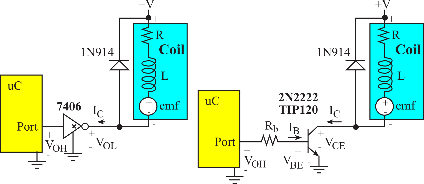
Figure 8.3.1. Binary interface to EM relay, solenoid, DC motor or speaker.
The second consideration is current. We must select the power supply and an interface device that can support the coil current. The 7406 is an open collector driver capable of sinking up to 40 mA. The 2N2222 is a bipolar junction transistor (BJT), NPN type, with moderate current gain. The TIP120 is a Darlington transistor, also NPN type, which can handle larger currents. **add links to data sheets** The IRF540 and IRLD024 are MOSFET transistors that can handle even more current. BJT and Darlington transistors are current-controlled (meaning the output is a function of the input current), while the MOSFET is voltage-controlled (output is a function of input voltage). When interfacing a coil to the microcontroller, we use information like Table 8.3.1 to select an interface device capable of the current necessary to activate the coil. It is good design practice to select a driver with a maximum current at least twice the required coil current. When the digital Port output is high, the interface transistor is active and current flows through the coil. When the digital Port output is low, the transistor is not active and no current flows through the coil.
The third consideration is inductance in the coil. The 1N914 diode in Figure 8.3.1 provides protection from the back emf generated when the switch is turned off, and the large dI/dt across the inductor induces a large voltage (on the negative terminal of the coil), according to V=L*dI/dt. For example, if you drive 0.1A through a 0.1 mH coil (Port output = 1) using a 2N2222, then disable the driver (Port output = 0), the 2N2222 will turn off in about 20ns. This creates a dI/dt of at least 5*106 A/s, producing a back emf of 500 V! The 1N914 diode shorts out this voltage, protecting the electronics from potential damage. The 1N914 used in this manner is called a snubber diode.
Because of the resistance of the coil, there will not be significant dI/dt when the device is turned on. Consider a DC motor as shown in Figure 8.3.1 with V= 12V, R = 50 Ω and L = 100 µH. Assume we are using a 2N2222 with a VCE of 1 V at saturation. Initially the motor is off (no current to the motor). At time t=0, the digital port goes from 0 to +3.3 V, and transistor turns on. Assume for this section, the emf is zero (motor has no external torque applied to the shaft) and the transistor turns on instantaneously, we can derive an equation for the motor (Ic) current as a function of time. The voltage across both LC together is 12-VCE = 11 V at time = 0+. At time = 0+, the inductor is an open circuit. Conversely, at time = ∞, the inductor is a short circuit. The Ic at time 0- is 0, and the current will not change instantaneously because of the inductor. Thus, the Ic is 0 at time = 0+. The Ic is 11V/50Ω= 220mA at time = ∞.
11 V = Ic *R +L*d Ic/dt
The general solution to this differential equation is
Ic = I0 + I1e-t/τ d Ic/dt = - (I1/τ)e-t/τ
We plug the general solution into the differential equation and boundary conditions.
11 V = (I0 + I1e-t/τ)*R -L*(I1/τ)e-t/τ
To solve the differential equation, the time constant will be τ = L/R = 2 µsec. Using initial conditions, we get
Ic = 220mA*(1- e-t/2µs)
|
Device |
Type |
Maximum current |
|
TM4C123 |
CMOS |
8 mA |
|
MSPM0 |
CMOS |
6 mA (2 pins with 20 mA) |
|
7406 |
TTL logic |
40 mA |
|
PN2222 |
BJT NPN |
150 mA |
|
2N2222 |
BJT NPN |
500 mA |
|
TIP120 |
Darlington NPN |
5 A |
|
IRLD024 |
power MOSFET |
2.5 A |
|
IRF540 |
power MOSFET |
28 A |
Table 8.3.1. Possible devices that can be used to interface a coil compared to the microcontroller.
Observation: It is important to realize that many devices cannot be connected directly up to the microcontroller. In the specific case of motors, we need an interface that can handle the voltage and current required by the motor.
If you are sinking 16 mA (IOL) with the 7406, the output voltage (VOL) will be 0.4V. However, when the IOL of the 7406 equals 40 mA, its VOL will be 0.7V. 40 mA is not a lot of current when it comes to typical coils. However, the 7406 interface is appropriate to control small relays.
: A relay is interfaced with the 7406 circuit in Figure 8.3.1. The positive terminal of the coil is connected to +5V, and the coil requires 40 mA. What will be the voltage across the coil when active?
For the 2N2222 and TIP120 NPN transistors, if the port output is low, no current can flow into the base, so the transistor is off, and the collector current, IC, will be zero. If the port output is high, current does flow into the base and VBE goes above VBEsat turning on the transistor. The transistor is in the linear range if VBE ≤ VBEsat and Ic = hfe*Ib. The transistor is in saturated mode if VBE ≥ VBEsat, VCE = 0.3V and Ic < hfe*Ib. We select the resistor for the NPN transistor interfaces to operate right at the transition between linear and saturated mode. We start with the desired coil current, Icoil (the voltage across the coil will be +V-VCE which will be about +V-0.3V). Next, we calculate the needed base current (Ib) given the current gain of the NPN
Ib = Icoil /hfe
knowing the current gain of the NPN (hfe), see Table 8.3.2. Finally, given the output high voltage of the microcontroller (VOH is about 3.3 V) and base-emitter voltage of the NPN (VBEsat) needed to activate the transistor, we can calculate the desired interface resistor.
Rb ≤ (VOH - VBEsat)/ Ib = hfe *(VOH - VBEsat)/ Icoil
The inequality means we can choose a smaller resistor, creating a larger Ib. Because the of the transistors can vary a lot, it is a good design practice to make the Rb resistor about ½ the value shown in the above equation. Since the transistor is saturated, the increased base current produces the same VCE and thus the same coil current.
With an N-channel switch, like Figure 8.3.1, current is turned on and off by connecting/disconnecting one side of the coil to ground, while the other side is fixed at the voltage supply. A second type of binary interface uses P-channel switches to connect/disconnect one side of the coil to the voltage supply, while the other side is fixed at ground, as shown in Figure 8.3.2. To activate a PNP transistor (e.g., PN2907 or TIP125), there must be a VEB greater than 0.7 V. To deactivate a PNP transistor, the VEB voltage must be 0. Because the transistor is a current amplifier, there must be a resistor into the base to limit the base current.
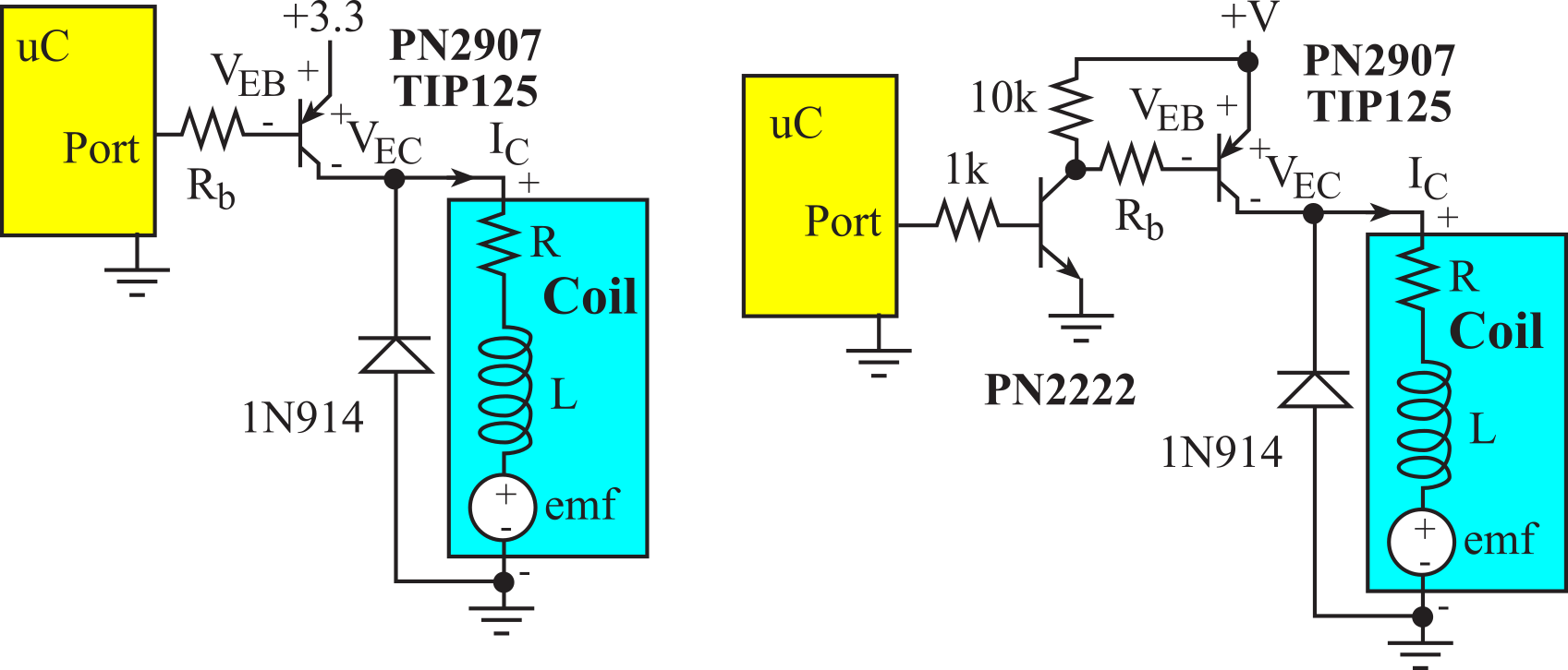
Figure 8.3.2. PNP interface to EM relay, solenoid, DC motor or speaker.
To understand how the PNP interface on the right of Figure 8.3.2 operates, consider the behavior for the two cases: the Port output is high, and the Port output is low. If the Port output is high, its output voltage will be between 2.4 and 3.3 V. This will cause current to flow into the base of the PN2222, and its Vbe will saturate to 0.7 V. The base current into the PN2222 could be from (2.4-0.7)/1000 to (3.3-0.7)/1000, or 1.7 to 2.6 mA. The microcontroller will be able to source this current. This will saturate the PN2222 and its VCE will be 0.3 V. This will cause current to flow out of the base of the PN2907, and its VEB will saturate to 0.7 V. If the supply voltage is V, then the PN2907 base current is (V-0.7-0.3)/Rb. Since the PNP transistor is on, VEC will be small and current will flow from the supply to the coil. If the port output is low, the voltage output will be between 0 and 0.4V. This is not high enough to activate the PN2222, so the NPN transistor will be off. Since there is no IC current in the PN2222, the 10k and Rb resistors will place +V at the base of the PN2907. Since the VEB of the PN2907 is 0, this transistor will be off, and no current will flow into the coil. For parameter values see Table 8.3.2.
|
Type |
NPN |
PNP |
package |
Vbe(SAT) |
Vce(SAT) |
hfe min/max |
Ic |
|
general purpose |
2N3904 |
2N3906 |
TO-92 |
0.85 V |
0.2 V |
100 |
10mA |
|
general purpose |
PN2222 |
PN2907 |
TO-92 |
1.2 V |
0.3 V |
100 |
150mA |
|
general purpose |
2N2222 |
2N2907 |
TO-18 |
1.2 V |
0.3 V |
100/300 |
500mA |
|
power transistor |
TIP29A |
TIP30A |
TO-220 |
1.3 V |
0.7 V |
15/75 |
1A |
|
power transistor |
TIP31A |
TIP32A |
TO-220 |
1.8 V |
1.2 V |
25/50 |
3A |
|
power transistor |
TIP41A |
TIP42A |
TO-220 |
2.0 V |
1.5 V |
15/75 |
3A |
|
power darlington |
TIP120 |
TIP125 |
TO-220 |
2.5 V |
2.0 V |
1000 min |
3A |
Table 8.3.2. Parameters of typical transistors used to source or sink current.
MOSFETs can handle significantly more current than BJT or Darlington transistors. MOSFETs are voltage-controlled switches. The difficulty with interfacing MOSFETs to a microcontroller is the large gate voltage needed to activate it. Figure 8.3.3 shows two N-channel interfaces. The IRLD024 can be controlled directly from a port pin (VGS>2V). The 10k resistor to the IRLD024 gate does not affect the on or off voltages but decreases dI/dt. The IRF540 requires a gate voltage above 7V to be fully active, therefore needs the BJT interface to boost the gate voltage. The IRF540 circuit operates in negative logic. When the port pin is high, the 2N2222 is active making the MOSFET gate voltage 0.3V (VCE of the PN2222). A VGS of 0.3V turns off the MOSFET. When the port pin is low, the 2N2222 is off making the MOSFET gate voltage +V (pulled up through the 10kΩ resistor). The VGS is +V, which turns the MOSFET on.
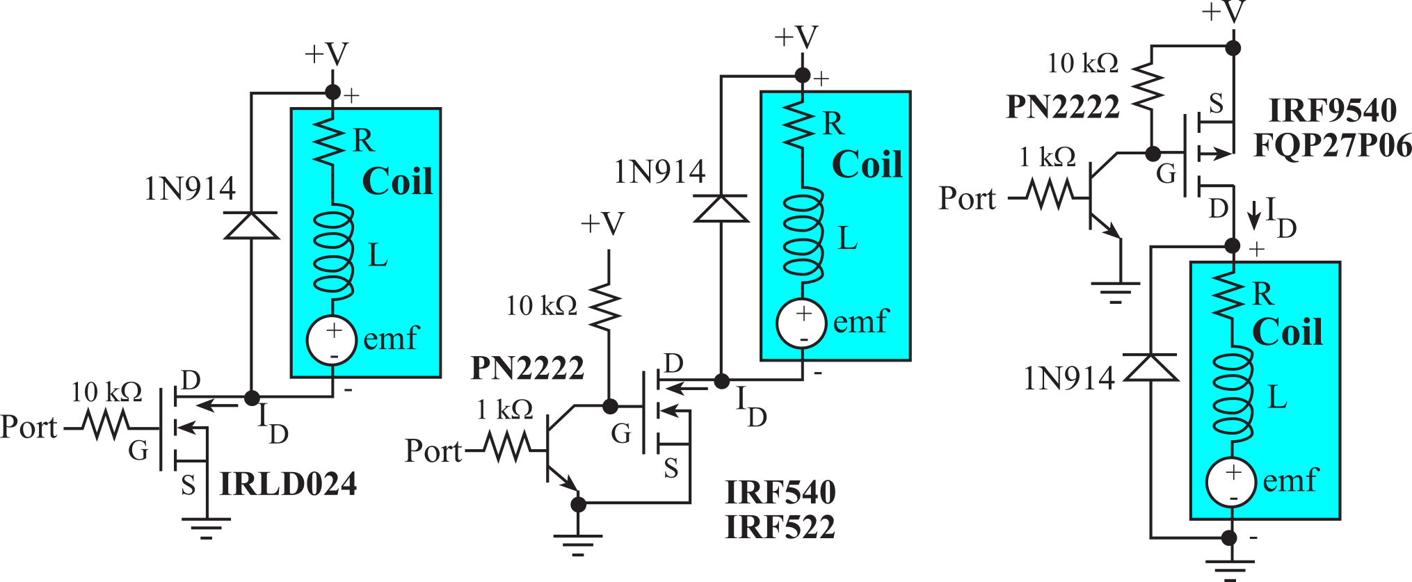
Figure 8.3.3. MOSFET interfaces to EM relay, solenoid, DC motor or speaker.
The right side of Figure 8.3.3 shows a P-channel MOSFET interface. The IRF9540 P-channel MOSFET can source up to 20A when the source-gate voltage is above 7V. The FQP27P06 P-channel MOSFET can source up to 27A when the source-gate voltage is above 6V. This circuit operates in positive logic. When the port pin is high, the 2N2222 is active making the MOSFET gate voltage 0.3V. This makes VSG equal to +V-0.3, which turns on the MOSFET. When the port pin is low, the 2N2222 is off. Since the 2N2222 is off, the 10kΩ pull-up resistor makes the MOSFET gate voltage +V. In this case VSG equals 0, which turns off the MOSFET.
An H-bridge uses four transistors, allowing current to flow in either direction. Each output is a totem-pole drive circuit with a transistor sink and source. The DRV8838 drives one motor and the DRV8848 drives two. The DRV8838 can take a motor voltage VM up to 11V and drive up to 1.8A. If EN is high, power will be applied to the motor. PH controls the direction of the current. The nSLEEP signal can be made low to place the driver into low-current mode. The DRV8848 can take a motor voltage VM up to 12V and drive up to 2A to each motor. The operation of the DRV8848 is described in Table 8.3.3.
Figure 8.3.4. An H-bridge can drive current in either direction.
|
xIN1 |
xIN2 |
xOUT1 |
xOUT2 |
Function (DC motor) |
|
0 |
0 |
Z |
Z |
Coast (fast decay) |
|
0 |
1 |
0V |
VM |
Reverse |
|
1 |
0 |
VM |
0 |
Forward |
|
1 |
1 |
0V |
0V |
Brake (slow decay) |
Table 8.3.3. Operation of the DRV8848, where x is A or B.
: When would you replace use a DRV8876 instead of a DRV8838?
8.3.2. Electromagnetic and Solid-State Relays
A relay is a device that responds to a small current or voltage change by activating switches or other devices in an electric circuit. It is used to remotely switch signals or power. The input control is usually electrically isolated from the output switch. The input signal determines whether the output switch is open or closed. Relays are classified into three categories depending upon whether the output switches power (i.e., high currents through the switch) or electronic signals (i.e., low currents through the switch). Another difference is how the relay implements the switch. An electromagnetic (EM) relay uses a coil to apply EM force to a contact switch that physically opens and closes. The solid-state relay (SSR) uses transistor switches made from solid state components to electronically allow or prevent current flow across the switch). The three types are
1. The classic general-purpose relay has an EM coil and can switch AC power
2. The reed relay has an EM coil and can switch low-level DC electronic signals
3. The solid-state relay (SSR) has an input triggered semiconductor power switch
Two solid state relays are shown in Figure 8.3.5. Interfacing an SSR is like interfacing an LED. SSRs allow the microcontroller to switch AC loads from 1 to 30A. They are appropriate in situations where the power is turned on and off many times.
Figure 8.3.5. Solid state relays can be used to control power to an AC appliance.
The input circuit of an EM relay is a coil with an iron core. The output switch includes two sets of silver or silver-alloy contacts (called poles.) One set is fixed to the relay frame, and the other set is located at the end of leaf spring poles connected to the armature. The contacts are held in the "normally closed" position by the armature return spring. When the input circuit energizes the EM coil, a "pull in" force is applied to the armature and the "normally closed" contacts are released (called break) and the "normally open" contacts are connected (called make.) The armature pull in can either energize or de-energize the output circuit depending on how it is wired. Relays are mounted in special sockets or directly soldered onto a PC board.
The number of poles (e.g., single pole, double pole, 3P, 4P etc.) refers to the number of switches that are controlled by the input. The relay shown below is a double pole because it has two switches. Single-throw means each switch has two contacts that can be open or closed. Double-throw means each switch has three contacts. The common contact will be connected to one of the other two contacts (but not both at the same time.) The parameters of the output switch include maximum AC (or DC) power, maximum current, maximum voltage, on resistance, and off resistance. A DC signal will weld the contacts together at a lower current value than an AC signal, therefore the maximum ratings for DC are considerable smaller than for AC. Other relay parameters include turn on time, turn off time, life expectancy, and input/output isolation. Life expectancy is measured in number of operations. Figure 8.3.6 illustrates the various configurations available. The sequence of operation is described in Table 8.3.4.
Figure 8.3.6. Standard relay configurations.
|
Form |
Activation Sequence |
Deactivation Sequence |
|
A |
Make 1 |
Break 1 |
|
B |
Break 1 |
Make 1 |
|
C |
Break 1, Make 2 |
Break 2, Make 1 |
|
D |
Make 1, Break 2 |
Make 2, Break 1 |
|
E |
Break 1, Make 2, Break 3 |
|
Table 8.3.4. Standard definitions for five relay configurations.
8.3.3. Solenoids
Solenoids are used in discrete mechanical control situations such as door locks, automatic disk/tape ejectors, and liquid/gas flow control valves (on/off type). Much like an EM relay, there is a frame that remains motionless, and an armature that moves in a discrete fashion (on/off). A solenoid has an electro-magnet. When current flows through the coil, a magnetic force is created causing a discrete motion of the armature. Each of the solenoids shown Figure 8.3.7 has a cylindrically-shaped armature the moves in the horizontal direction relative to the photograph. The solenoid on the top is used in a door lock, and the second from top is used to eject the tape from a video cassette player. When the current is removed, the magnetic force stops, and the armature is free to move. The motion in the opposite direction can be produced by a spring, gravity, or by a second solenoid.
Figure 8.3.7. Photo of four solenoids.
8.3.4. Brushed DC Motor
Like the solenoid and EM relay, the brushed DC motor has a frame that remains motionless (called the stator), and an armature that moves (called the rotor). The motor has an electromagnetic coil as well, located on the rotor, and the rotor is positioned inside the stator. In Figure 8.3.8, North and South refer to a permanent magnet, generating a constant B field from left to right. In this case, the rotor moves in a circular manner. When current flows through the coil, a magnetic force is created causing a rotation of the shaft. A brushed DC motor uses commutators to flip the direction of the current in the coil. In this way, the coil on the right always has an up force, and the one on the left always has a down force. Hence, a constant current generates a continuous rotation of the shaft. When the current is removed, the magnetic force stops, and the shaft is free to rotate. In a pulse-width modulated interface, the computer activates the coil with a voltage of fixed magnitude but varies the duty cycle to adjust the power delivered to the motor.
Figure 8.3.8. A brushed DC motor uses a commutator to flip the coil current.
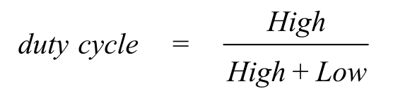
With a simple GPIO pin the microcontroller can only control electrical power to a device in a binary fashion: either all on or all off. Sometimes it is desirable for the microcontroller to be able to vary the delivered power in a variable manner. One effective way to do this is to use pulse width modulation (PWM). The basic idea of PWM is to create a digital output wave of fixed frequency but allow the microcontroller to vary its duty cycle. The system is designed in such a way that High+Low is constant (meaning the frequency is fixed). The duty cycle is defined as the fraction of time the signal is high:
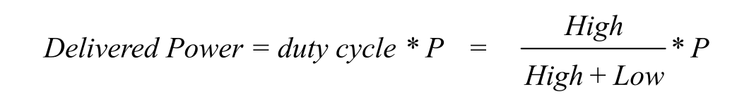
Hence, duty cycle varies from 0 to 1. We interface this digital output wave to an external actuator (like a DC motor), such that power is applied to the motor when the signal is high, and no power is applied when the signal is low. We purposely select a frequency high enough, so the DC motor does not start/stop with each individual pulse but rather responds to the overall average value of the wave. The average value of a PWM signal is linearly related to its duty cycle and is independent of its frequency. Let P (P=V*I) be the power to the DC motor when the control signal is high. Under conditions of constant speed and constant load, the delivered power to the motor is linearly related to duty cycle.
Unfortunately, as speed and torque vary, the developed emf will affect delivered power. Nevertheless, PWM is a very effective mechanism, allowing the microcontroller to adjust delivered power.
A DC motor has an electro-magnet as well. When current flows through the coil, a magnetic force is created causing a rotation of the shaft. Brushes positioned between the frame and armature are used to alternate the current direction through the coil, so that a DC current generates a continuous rotation of the shaft. When the current is removed, the magnetic force stops, and the shaft is free to rotate. The resistance in the coil (R) comes from the long wire that goes from the + terminal to the - terminal of the motor. The inductance in the coil (L) arises from the fact that the wire is wound into coils to create the electromagnetics. The coil itself can generate its own voltage (emf) because of the interaction between the electric and magnetic fields. If the coil is a DC motor, then the emf is a function of both the speed of the motor and the developed torque (which in turn is a function of the applied load on the motor.) Because of the internal emf of the coil, the current will depend on the mechanical load. For example, a DC motor running with no load might draw 50 mA, but under load (friction) the current may jump to 500 mA.
Figure 8.3.9 shows the speed versus power of 10 motors of the same type. Notice three characteristics from this data:
• None of the motors spin with power equal to 100 mW,
• All ten are different, meaning to control speed we need a tachometer,
• The speed versus power is not linear.
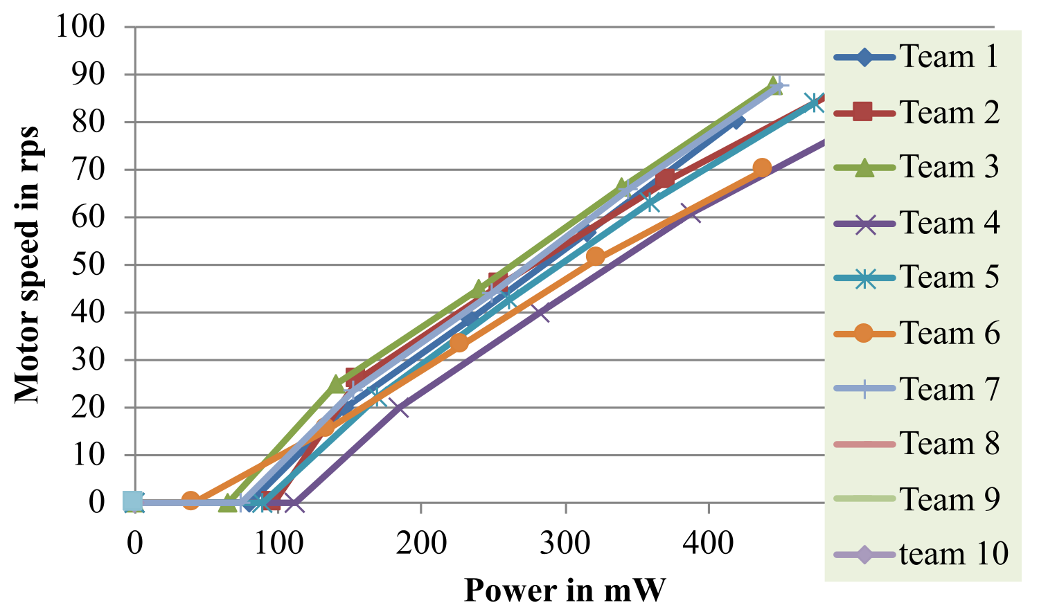
Figure 8.3.9. Speed versus power for 10 motors.
Torque is defined as force times distance. When a DC motor is moving a robot, force is applied at the wheel-floor surface, causing the robot to move. Distance is the radius of the robot wheel. Friction induces an emf in the motor, as defined in Figure 8.3.8. Increasing the friction (mechanical load) will make the emf more negative, increasing the current through the motor and its electrical interface.
There is power threshold above which the driver must supply to cause a stopped motor to begin spinning. This threshold is between 100 and 150 mW for the motors in Figure 8.3.9. Stiction (a combination of the words static and friction) is the force that needs to be overcome to enable relative motion of stationary objects in contact. Any solid objects pressing against each other (but not sliding) will require some threshold of force parallel to the surface of contact in order to overcome static adhesion. Stiction is a threshold, not a continuous force. However, stiction might also be an illusion made by the rotation of kinetic friction. Another name for stiction is holding torque. Reference wikipedia.
Motor power, measured in watts or horsepower, quantifies the rate at which a motor performs work. Power is rotational speed (angular velocity) times torque output. Figure 8.3.10 shows the motor torque is inversely related to motor speed. The maximum power occurs when the speed is ½ the no load speed, and the torque is ½ the stall torque.

Figure 8.3.10. Torque versus speed.
There are six considerations when selecting a DC motor: speed, torque, voltage, current, size, and weight. Speed is the rate in rotations per minute (RPM) that the motor will spin, and torque is the available force times distance the motor can provide at that speed. We select the motor voltage to match the available power supply. Unlike LEDs, we MUST not use a resistor in series with a motor to reduce the voltage. In general, the motor voltage matches the power supply voltage. When interfacing we will need to know maximum current.
8.3.5. Robot Systems Learning Kit (RSLK2)
The original RSLK was designed for Texas Instruments based on the MSP432 microcontroller. Since the MSP432 went out of production, getting MSP432 LaunchPads for this version of the robot has been difficult.
The robot has been redesigned for either the TM4C123 or the MSPM0G3507 LaunchPad. The RSLK2 robot has two independent drive wheels, and a third castor for stability. Each wheel is driven by a 7.2-V 0.5-A geared DC motor. See Figure 8.3.11.
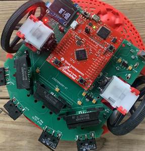
Figure 8.3.11. Robot Systems Learning Kit (RSLK2).
The two motors are driven by a dual H-bridge using either an L293D Darlington or a DRV8847 MOSFET. Both chips include snubber diodes to suppress the back EMF induced by the inductance of the motor. The dual H-bridge allows the software to independently control the power and direction of each wheel. The DRV8847 can drive up to 1 A, while the L293D can drive only 600 mA. L293D comes in a DIP package and thus is easier to solder. The period of the PWM output is chosen to be 2 ms, which is about 10 times shorter than the time constant of the motor. The electronic driver will turn on and off at this rate, but the motor only responds to the average level. The software sets the duty cycle of the PWM to adjust the delivered power. Let H+L=40000 be the fixed period of the PWM interface. When active, the interface will drive +7 V across the motor. The current will be a function of the friction applied to the shaft. There are four modes of the RSLK robot. To make the wheel rotate forward, we set the DIR pin low and run the PWM at high for H and low for L. To make the wheel rotate backward, we set the DIR pin high and run the PWM at high for L and low for H. See Table 8.3.5.
|
Robot mode |
PF3 |
PA2 |
PF2 |
PA3 |
|
Forward |
PWM = H |
0 |
PWM = H |
0 |
|
Backward |
PWM = L |
1 |
PWM = L |
1 |
|
Turn right |
PWM = L |
1 |
PWM = H |
0 |
|
Turn left |
PWM = H |
0 |
PWM = L |
1 |
Table 8.3.5. Control signals for the two DC motors.
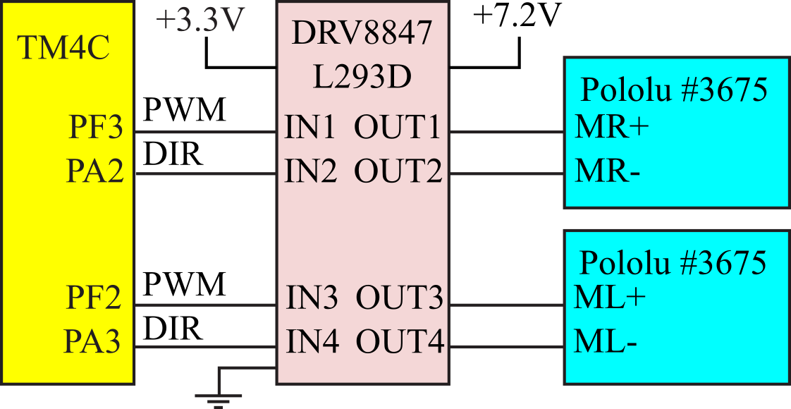
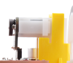
Figure 8.3.12. DC motor interface for the RSLK2 robot using a DRV8847.
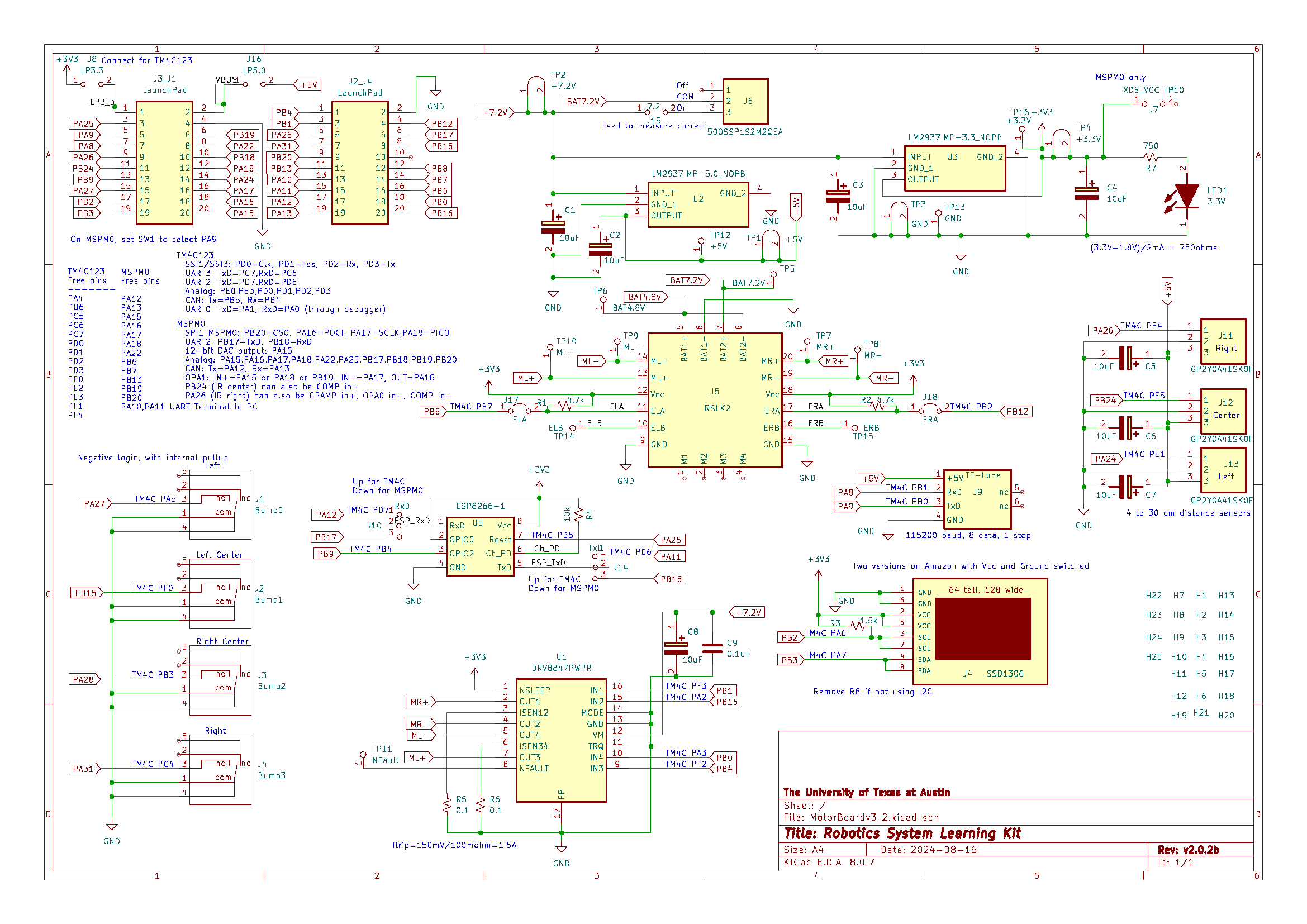
Figure 8.3.13. Circuit for the RSLK2 robot.
8.3.6. Brushless DC Motor (BLDC)
A brushless DC motor (BLDC), as the name implies, does not have mechanical commutators or brushes to flip the currents. It is a synchronous electric motor powered by direct current and has an electronic commutation system, rather than a mechanical commutator and brushes. In BLDC motors, current-to-torque and voltage-to-rpm are linear relationships. The controller uses either the back emf of the motor itself or Hall-effect sensors to know the rotational angle of the shaft. The controller uses this angle to set the direction of the currents in the electromagnets, shown as the six step sequence in Figure 8.3.14. Other differences from a brushed DC motor are that the BLDC permanent magnets are in the rotor and the electromagnets are in the stator. Typically, there are three electromagnetic coils, labeled Phase A, Phase B, and Phase C, which are arranged in a Wye formation. Each coil can be modeled as a resistance, inductance, and emf, as previously shown in Figure 8.3.3. The Hall sensor goes through the sequence 001, 000, 100, 110, 111, 011 each time the shaft rotates once. It is a synchronous motor because the controller adjusts the phase current according to the six-step sequence. For example, if the Hall sensor reads 001, then the controller places +V on Phase A and ground on Phase C (step 1). In other words, the phase currents are synchronized to the shaft position. To rotate the motor in the other direction, we reverse the currents in each step. We will see later for stepper motors that the process is reversed. For stepper motors, the controller sets the phase currents and the motor moves to that position. To adjust the power to a BLDC motor, we change the voltage, V, or use PWM on the control signals themselves. The PWM period should be at least 10 times shorter than the time for each of the six steps. In other words, the PWM frequency should be 60 times faster than the shaft rotational frequency.
BLDC motors have many advantages and few disadvantages when compared to brushed DC motors. Because there are no brushes, they require less maintenance and hence have a longer life. Therefore, they are appropriate for applications where servicing is inconvenient or expensive. BLDC motors produce more output torque per weight than brushed DC motors and hence are used for pilotless airplanes and helicopters. Because the rotor is made of permanent magnets, the rotor inertia is less, allowing it to spin faster and to change quicker. In other words, it has faster acceleration and deceleration. Removing the brushes reduces friction, which also contributes to the improved speed and acceleration. It has a linear speed/torque relationship. Because there is no brush contact, BLDC motors operate more quietly and have less Electromagnetic Interference (EMI). The only disadvantages are the complex controller and increased cost.
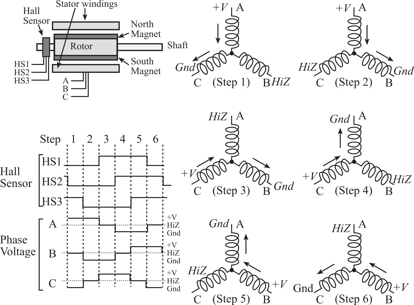
Figure 8.3.14. A brushless DC motor uses an electronic commutator.
Interface a 24-V 2-A brushless DC motor. A brushless DC motor has three coils connected in a Wye pattern. Each of the phases can be driven into one of three states: 24 V, ground, or floating. We will use MOSFETs to source and sink the current required by the motor (Figure 8.3.15). Remember, when the motor is under load, the current will increase. The P-channel MOSFET will connect the 24 V to the phase when its gate voltage is below 24 V. The N-channel MOSFET will drive the phase to ground when its gate is above zero. It will be important to prevent turning on both MOSFETs at the same time. For safety reasons, we will use digital logic in the interface so the driver can only be in the three valid states. Table 8.3.6 shows the design specification for Phase A. When EnA is low, both MOSFETs are off and the phase will float (HiZ). When EnA is high, the InA determines whether the phase is high or low. The six gate voltages are labeled in Figure 8.3.15 as G1 to G6. These gate voltages are 24 V, produced by the 10 kΩ pull-up, when the corresponding 7406 driver output is floating. Alternatively, these gate voltages are 0.5 V when the 7406 driver output is low. It is good design to use integrated drivers like the ULN2074, L293, TPIC0107, and MC3479 rather than individual transistors. In particular, the entire interface circuit in Figure 8.3.15 could be replaced with three L6203 full bridge drivers.
|
EnA |
InA |
G1 |
G2 |
P-chan |
N-chan |
Phase A |
|
1 |
1 |
Low |
Low |
On |
Off |
+24 V |
|
1 |
0 |
High |
High |
Off |
On |
Ground |
|
0 |
X |
High |
Low |
Off` |
Off |
HiZ |
Table 8.3.6. Control signals for one phase of the brushless DC motor.

Figure 8.3.15. Brushless DC motor interface.
The InA, InB, and InC signals in Figure 8.3.15 can be connected to any GPIO output, whereas the EnA, EnB, and EnC signals will be attached to PWM outputs. The PWM period will be selected 60 times faster than the motor speed in rps. The three Hall-effect sensor signals will be attached to input capture pins. Interrupts will be armed for both the rise and fall of these three sensors. In this way, an ISR will be run at the beginning of each of the six steps. The BLDC motor is a synchronous motor, so the six control signals are a function of the shaft position. In particular, the ISR will look up the Hall sensors and output the pattern, as shown in Table 8.3.7.
|
Step |
HS1 |
HS2 |
HS3 |
EnA |
InA |
EnB |
InB |
EnC |
InC |
A |
B |
C |
|
1 |
0 |
0 |
1 |
PWM |
1 |
0 |
X |
PWM |
0 |
24V |
HiZ |
0V |
|
2 |
0 |
0 |
0 |
PWM |
1 |
PWM |
0 |
0 |
X |
24V |
0V |
HiZ |
|
3 |
1 |
0 |
0 |
0 |
X |
PWM |
0 |
PWM |
1 |
HiZ |
0V |
24V |
|
4 |
1 |
1 |
0 |
PWM |
0 |
0 |
X |
PWM |
1 |
0V |
HiZ |
24V |
|
5 |
1 |
1 |
1 |
PWM |
0 |
PWM |
1 |
0 |
X |
0V |
24V |
HiZ |
|
6 |
0 |
1 |
1 |
0 |
X |
PWM |
1 |
PWM |
0 |
HiZ |
24V |
0V |
Table 8.3.7. Input-output relationships for the synchronous controller.
Furthermore, when any of the enable signals are scheduled to be high, they will be pulsed using positive logic PWM. The software can adjust the delivered power to the BLDC motor by setting the duty cycle of the PWM.
: How do the waveforms in Figure 8.3.14 change if we are running at 50% power?
8.3.7. Stepper Motors
Stepper motors are very popular for microcontroller-controlled machines because of their inherent digital interface. It is easy for a microcontroller to control both the position and velocity of a stepper motor in an open loop fashion. Although the cost of a stepper motor is typically higher than an equivalent DC permanent magnetic field motor, the overall system cost is reduced because stepper motors may not require feedback sensors. For these reasons, they are used in many computer peripherals such as hard disk drives, scanners, and printers. Figure 8.3.16 shows a stepper motor is made with EM coils and permanent magnets (teeth).
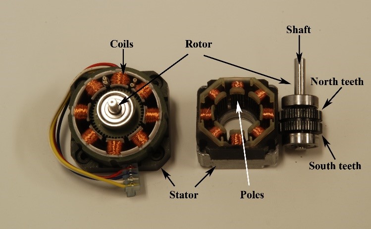
Figure 8.3.16. Stepper motors have permanent magnets on the rotor and electromagnetics around the stator.
For
information on stepper motors see these data sheets
StepperBasic.pdf
StepperDriveBasic.pdf
StepperSelection.pdf
Stepper.pdf
Stepper_ST.pdf
Figure 8.3.17 shows a simplified stepper motor. The permanent magnet stepper has a rotor and a stator. The rotor is manufactured from a gear-shaped permanent magnet. This simple rotor has one North tooth and one South tooth. The stator consists of multiple iron-core electromagnets whose poles are also equally spaced. The stator of this simple stepper motor has four electromagnets and four poles.
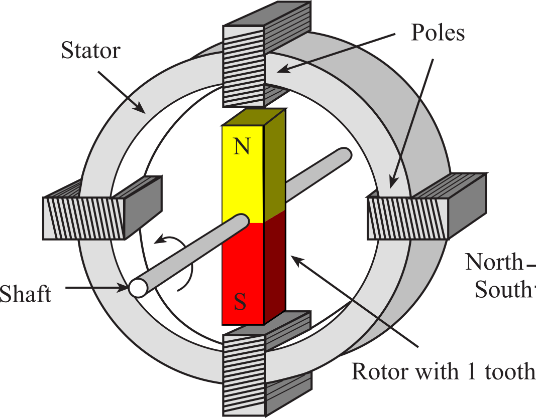
Figure 8.3.17. Simple stepper motor that has 4 steps/revolution.
The operation of this simple stepper motor is illustrated in Figure 8.3.18. In general, if there are n North teeth and n South teeth, the shaft will rotate 360°/(4*n) per step. For this simple motor, each step causes 90° rotation.
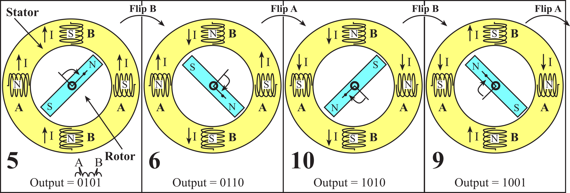
Figure 8.3.18. The full-step sequence to rotate a stepper motor.
Click 'CW' or 'CCW' to step the motor clockwise and counterclockwise, respectively. Observe how different microcontroller outputs to the motor coils produce different responses from the motor. Assume that an output value of '1' to a motor coil will cause current to flow in that motor, resulting in a 'N' oriented magnetic field at that coil.
Output=0101. Assume the initial position is the one on the left with the output equal to 0101. There are strong attractive forces between North and South magnets. This is a stable state because the North tooth is equally positioned between the two South electromagnets, and the South tooth is equally positioned between the two North electromagnets. There is no net torque on the shaft, so the motor will stay fixed at this angle. In fact, if there is an attempt to rotate the shaft with an external torque, the stepper motor will oppose that rotation and try to maintain the shaft angle fixed at this position. In fact, stepper motors are rated according to their holding torque. Typical holding torques range from 10 to 300 oz-in.
Output=0110. When the software changes the output to 0110, the polarity of Phase B is reversed. The rotor is in an unstable state, because the North tooth is near the North electromagnet on the top, and the South tooth is near the South electromagnet on the bottom. The rotor will move because there are strong repulsive forces from the top and bottom poles. By observing the left and right poles, the closest stable state occurs if the rotor rotates clockwise, resulting in the stable state illustrated as the picture in Figure 8.3.18 labeled "Output=0110". The "Output=0110" state is exactly 90° clockwise from the "Output=0101" state. Now, once again the North tooth is near the South poles and the South tooth is near the North poles. This new position has strong attractive forces from all four poles, holding the rotor at this new position.
Output=1010. Next, the software outputs 1010, causing the polarity of Phase A to be reversed. This time, the rotor is in an unstable state because there are strong repulsive forces on the left and right poles. The closest stable state occurs if the rotor rotates clockwise, resulting in the stable state illustrated in the picture Figure 8.3.18 labeled as "Output=1010". This new state is exactly 90° clockwise from the last state, moving to position the North tooth near the South poles and the South tooth near the North poles.
Output=1001. When the software outputs 1001, the polarity of Phase B is reversed. This causes a repulsive force on the top and bottom poles and the rotor rotates clockwise again by 90°, resulting in the stable state shown as the picture labeled "Output=1001". After each change in software, there are two poles that repel and two poles that attract, causing the shaft to rotate. The rotor moves until it reaches a new stable state with the North tooth close to South poles and the South tooth close to North poles. When the software outputs a 0101, it will rotate 90° resulting in a position like the original "Output=0101" state. If the software outputs a new value from the 5,6,10,9 sequence every 250 ms, the motor will spin clockwise at 1 rps. The rotor will spin in a counterclockwise direction if the sequence is reversed.
To provide for finer control over the rotation we use a stepper with more teeth and more poles. Figure 8.3.18 shows a rotor with 12 North teeth and 12 South teeth. The teeth are equally spaced and offset from each other by half the tooth pitch. A stepper motor with this rotor will have 48 steps per revolution, or 7.5°/step.
Figure 8.3.19. A rotor with 12 teeth.
The stepper motors in Figure 8.3.16 have 50 North teeth and 50 South teeth, resulting in motors with 200 steps per revolution. The stator of a stepper motor with 200 steps per revolution has eight electromagnets each with five poles, making a total of 40 poles.
Observation: If there are m North teeth and m South teeth, there will be n=4m steps per revolution, and the step angle θ=360°/n.
There is an eight-number sequence called half-stepping. In full stepping, the direction of current in one of the coils is reversed in each step. In half-stepping, the coil goes through a no-current state between reversals. The half-stepping sequence is 0101, 0100, 0110, 0010 1010, 1000, 1001, and 0001. If a coil is driven with the 00 command, it is not energized, and the electromagnet applies no force to the rotor. A motor that requires 200 full steps to rotate once will require 400 half-steps to rotate once. In other words, the half-step angle is ½ of a full-step angle.
In a four-wire (or bipolar) stepper motor, the electromagnets are wired together, creating two phases. The five- and six-wire (or unipolar) stepper motors also have two phases, but each is center-tapped to simplify the drive circuitry. In a bipolar stepper all copper in the windings carries current at all times; whereas in a unipolar stepper, only half the copper in the windings is used at any one time.
To spin the stepper motor at a constant speed the software outputs the 5-6-10-9 sequence separated by a fixed time between outputs. This is an example of blind-cycle interfacing, because there is no feedback from the motor to the software giving the actual speed and/or position of the motor. If Δt is the time between outputs in seconds, and the motor has n steps per revolution, the motor speed will be 60/(n*Δt) in RPM.
The time between states determines the rotational speed of the motor. Let Δt be the time between steps. Let θ be the step angle then the rotational velocity, v, is θ/Δt. If the load on the shaft is below the holding torque of the motor, the position and speed can be reliably maintained with an open loop software control algorithm. To prevent slips (digital commands that produce no rotor motion) it is important to limit the change in acceleration defined as jerk. Let ∆t(n-2), Δt(n-1), Δt(n) be the discrete sequence of times between steps. The instantaneous rotational velocity is given by
v(n) = θ/∆t
The acceleration is given by
a(n) = (v(n) - v(n-1))/∆t(n) =(θ/∆t(n) - θ/∆t(n-1))/∆t(n) =θ/∆t(n)2 - θ/(∆t(n-1)∆t(n))
The change in acceleration, or jerk, is given by
b(n) =(a(n) - a(n-1))/∆t(n)
For example, if the time between steps is to be increased from 1000 to 2000 µs, an ineffective approach as shown in Table 8.3.8 would be simply to go directly from 1000 to 2000. This produces a very large jerk that may cause the motor to slip.
|
n |
∆t (µs) |
v(n) (°/sec) |
a(n) (°/sec2) |
b(n) (°/sec3) |
|
1 |
1000 |
1800 |
|
|
|
2 |
1000 |
1800 |
0.00E+00 |
|
|
3 |
2000 |
900 |
-2.50E+05 |
0.00E+00 |
|
4 |
2000 |
900 |
0.00E+00 |
-2.25E+08 |
|
5 |
2000 |
900 |
0.00E+00 |
2.25E+08 |
|
6 |
2000 |
900 |
0.00E+00 |
0.00E+00 |
Table 8.3.8. An ineffective approach to changing motor speed.
Table 8.3.9 shows that a more gradual change from 1000 to 2000 produces a 10 times smaller jerk, reducing the possibility of slips. The optimal solution (the one with the smallest jerk) occurs when v(t) has a quadratic shape. This will make a(t) linear, and b(t) a constant. Limiting the jerk is particularly important when spinning up a stopped motor.
|
n |
∆t (µs) |
v(n) (°/sec) |
a(n) (°/sec2) |
b(n) (°/sec3) |
|
1 |
1000 |
1800 |
|
|
|
2 |
1000 |
1800 |
0.00E+00 |
|
|
3 |
1000 |
1800 |
0.00E+00 |
0.00E+00 |
|
4 |
1008 |
1786 |
-1.39E+04 |
-1.38E+07 |
|
5 |
1032 |
1744 |
-4.11E+04 |
-2.64E+07 |
|
6 |
1077 |
1671 |
-6.77E+04 |
-2.47E+07 |
|
7 |
1152 |
1563 |
-9.37E+04 |
-2.26E+07 |
|
8 |
1275 |
1411 |
-1.19E+05 |
-1.96E+07 |
|
9 |
1500 |
1200 |
-1.41E+05 |
-1.48E+07 |
|
10 |
1725 |
1044 |
-9.06E+04 |
2.91E+07 |
|
11 |
1848 |
974 |
-3.78E+04 |
2.86E+07 |
|
12 |
1923 |
936 |
-1.96E+04 |
9.44E+06 |
|
13 |
1968 |
915 |
-1.09E+04 |
4.43E+06 |
|
14 |
1992 |
904 |
-5.65E+03 |
2.63E+06 |
|
15 |
2000 |
900 |
-1.77E+03 |
1.94E+06 |
|
16 |
2000 |
900 |
0.00E+00 |
8.85E+05 |
|
17 |
2000 |
900 |
0.00E+00 |
0.00E+00 |
Table 8.3.9. An effective approach to changing motor speed.
The bipolar stepper motor can be controlled with two H-bridge drivers. The L293 is a simple IC for interfacing stepper motors. It uses Darlington transistors in a double H-bridge configuration (as shown in Figure 8.3.20), which can handle up to 1 A per channel and voltages from 4 to 36 V. The L293D includes internal snubber diodes, but can only drive 600mA. The DRV8848 MOSFET H-bridge, shown in Figure 8.3.4, could also drive a bipolar stepper motor.
Figure 8.3.20. Bipolar stepper motor interface using a L293 driver.
The 1N914 snubber diodes protect the electronics from the back EMF generated when currents are switched on and off. The L293D has internal snubber diodes, but it can handle only 600 mA. Figure 8.3.20 shows four digital outputs from the microcontroller connected to the 1A, 2A, 3A, 4A inputs. The software rotates the stepper motor using either the standard full-step (5-6-10-9...) or half-step (5-4-6-2-10-8-9-1...) sequence.
The unipolar stepper architecture provides for bi-directional currents by using a center tap on each phase, as shown in Figure 8.3.21. The center tap is connected to the +V power source. An H bridge is not needed because the four coils need to be driven low (current flows) or floating (no current). The four ends of the phases are controlled with open collector drivers in the ULN2003B. If the base (B) is high, the collector (C) is connected to the emitter (E), and current flows through the coil. If the base (B) is low, the collector (C) floats, and no current flows through the coil. Each of the Darlington transistors on the ULN2003B has an internal snubber diode connected to the COM pin. The ULN2003B provides up to 500mA current.
Figure 8.3.21. Unipolar stepper motor interface using a ULN2003B.
Observation: Because only half of the electromagnets on a unipolar stepper are energized at one time, unipolar steppers have less torque when compared to a similar sized bipolar stepper.
: What changes could you make to a stepper motor system to increase torque, increasing the probability that a step command actually rotates the shaft?
: Do you need sensor feedback to measure the shaft position when using a stepper motor?
There are nine considerations when selecting a stepper motor: speed, torque, holding torque, bipolar/unipolar, voltage, current, steps/rotation, size, and weight. The first two parameters are speed and torque. Speed is the rate in rotations per minute (RPM) that the motor will spin, and torque is the available force times distance the stepper motor can provide at that speed. Stepper motors also have a holding torque, which is the force times distance that the motor will remain stopped when the input pattern is constant. We select the motor voltage to match the available power supply. Unlike LEDs, we MUST NOT use a resistor in series with a motor to reduce the voltage. This is because the impedance (Z=V/I) across a motor coil is not constant. In general, we choose the power supply voltage to match the needed motor voltage. We also need to know maximum current. We choose a bipolar stepper for situations where speed, torque, and efficiency are important. Unipolar steppers are appropriate for low-cost systems. If we are trying to control shaft angle it will be better to have a motor with more steps per rotation.
Example 8.3.1: Interface a 12-V, 200-mA stepper motor. The motor has 200 steps per revolution. Interface two switches, such that pressing one switch makes it spin clockwise, and pressing the other switch makes it spin counterclockwise.
Solution: The computer can make the motor spin by outputting the sequence ...,10,9,5,6,10,9,5,6,... over and over. For a motor with 200 steps/revolution each new output will cause the motor to rotate 1.8°. If the time in between outputs is fixed at ∆t seconds, then the shaft rotation speed will be 0.005/∆t in rps. We will connect the stepper motor interface to four output pins PB3-0. We will we connect the two positive logic switches on two input pins PB7-6. A bipolar stepper interface was shown in Figure 8.3.20, and the unipolar interface was shown in Figure 8.3.21, with the motor voltage +V set to 12 V. We define the active state of the coil when current is flowing. The basic operation is summarized in Table 8.3.10.
|
Port B output |
A1 |
A2 |
B1 |
B2 |
|
10 |
Activate |
Deactivate |
Activate |
Deactivate |
|
9 |
Activate |
Deactivate |
Deactivate |
Activate |
|
5 |
Deactivate |
Activate |
Deactivate |
Activate |
|
6 |
Deactivate |
Activate |
Activate |
Deactivate |
Table 8.3.10 Stepper motor sequence.
We will implement the software controller using a finite state machine (FSM). This approach yields a solution that is easy to understand and change. If the computer outputs the sequence backwards then the motor will spin in the other direction. In ensure proper operation, this ...,10,9,5,6,10,9,5,6,... sequence must be followed. For example, assume the computer outputs ..., 9, 5, 6, 10, and 9. Now it wishes to reverse direction, since the output is already at 9, then it should begin at 10, and continue with 6, 5, 9, ... In other words, if the current output is "9" then the only two valid next outputs would be "5" if it wanted to spin clockwise or "10" if it wanted to spin counterclockwise. Maintaining this proper sequence will be guaranteed by the state transition graph, see Figure 8.3.22.
Figure 8.3.22. A state transition graph (STG) used to control the stepper motor.
Program 8.3.1 shows the high-level software, and Program 8.3.2 shows the low-level software specific to the microcontroller and pin selection. Notice the 1-1 correspondence between the STG (Figure 8.3.22) and the STT (fsm[4] software). The constant OFFSET is chosen to create a 100ms interrupt period.
#define T100msec (8000000-OFFSET)
struct State{
uint8_t Out;
uint32_t Delay;
const struct State *Next[4];
};
typedef const struct State State_t;
#define S5 &fsm[0]
#define S6 &fsm[1]
#define S10 &fsm[2]
#define S9 &fsm[3]
State_t fsm[4]={
{5, T100msec, S5, S6, S9, S5},
{6, T100msec, S9,S10, S5, S6},
{10,T100msec,S10, S9, S6,S10},
{9, T100msec, S9, S5,S10, S9}
};
State_t *Pt; // Current State
void SysTick_Handler(void){ uint32_t Input;
Input = Switch_Input(); // 0,1,2,3
Pt = Pt->Next[Input]; // Next
Stepper_Output(Pt->Out); // Output
SysTick_Restart(Pt->Delay);
}
int main(void){ uint32_t Input;
Pt = &fsm[0]; // Initial state
SysTick_Init();
Stepper_Init(); // GPIO output to stepper, input from switches
while(1){
// other tasks
}
}
Program 8.3.1. FSM controller for the stepper motor.
|
// TM4C123 void Stepper_Init(void){ volatile uint32_t delay; DisableInterrupts(); PLL_Init(Bus80MHz); SYSCTL_RCGCGPIO_R |= 0x02; delay = SYSCTL_RCGCGPIO_R; GPIO_PORTB_PCTL_R &= ~0xFF00FFFF; GPIO_PORTB_DIR_R |= 0x0F; GPIO_PORTB_DIR_R &= ~0xC0; GPIO_PORTB_AFSEL_R &= ~0xCF; GPIO_PORTB_DR8R_R |= 0x0F; GPIO_PORTB_DEN_R |= 0xCF; EnableInterrupts(); } void Stepper_Output(uint32_t data){ GPIO_PORTB_DATA_R = (GPIO_PORTB_DATA_R&(~0x0F))|data; } uint32_t Switch_Input(void){ return (GPIO_PORTB_DATA_R&0xC0)>>6; } void SysTick_Restart(uint32_t time){ NVIC_ST_RELOAD_R = time; NVIC_ST_CURRENT_R = 0; } |
// MSPM0G3507 void Stepper_Init(void){ __disable_irq(); Clock_Init80MHz(0); LaunchPad_Init(); IOMUX->SECCFG.PINCM[PB7INDEX] = 0x00040081; IOMUX->SECCFG.PINCM[PB6INDEX] = 0x00040081; IOMUX->SECCFG.PINCM[PB3INDEX] = 0x00000081; IOMUX->SECCFG.PINCM[PB2INDEX] = 0x00000081; IOMUX->SECCFG.PINCM[PB1INDEX] = 0x00000081; IOMUX->SECCFG.PINCM[PB0INDEX] = 0x00000081; GPIOB->DOE31_0 |= 0x0F; __enable_irq(); }
void Stepper_Output(uint32_t data){ GPIOB->DOUT31_0 = (GPIOB->DOUT31_0&(~0x0F))|data; } uint32_t Switch_Input(void){ return (GPIOB->DIN31_0&0xC0)>>6; } void SysTick_Restart(uint32_t time){ SysTick->LOAD = time; SysTick->VAL = 0; } |
Program 8.3.2. Low-level software for the stepper motor.
To see a stepper motor robot, see Section 10.3
Controlling time is an important function of an
embedded system. One of the methods software can perform to set the
delivered power to an external device is pulse width modulation
(PWM). The basic idea is to oscillate an output so fast the external
device does not respond to the individual on and off events. Rather, the
delivered power will be a function of the average, called duty cycle.
Let H be the time the output is high, and L the time the output is low.
For PWM we will set P=H+L as a constant, and adjust H and L. The duty
cycle is defined as
Duty Cycle = H/(H+L)
The microcontroller has a rich set of built in functionality to product PWM signals. For details on the TM4C123 see Section T.8.
The human eye can see a flashing LED up to about 10
Hz. If we flash the LED at 100 Hz, our eyes will see a constant light, but
the brightness of the LED will depend linearly on the duty cycle. In
particular if the LED operating point is Vd, Id,
the LED power will be
Power = Vd*Id*H/(H+L)
Program 8.4.1 presents a simple PWM output. Notice that
this implementation uses all the processor time. H can vary from 4 to 799996 bus cycles,
while L varies from 799996 to 4. H+L should be constant, in this example 800,000*12.5ns = 10ms.
int main(void){
Clock_Init80MHz(0);
LED_Init(); // PB1 output
while(1){
LED_On(); // PB1=1
Delay(600000);
LED_Off(); // PB1=0
Delay(200000);
}
}
Program 8.4.1. Software implementation of 75% PWM.
: If H+L=100000, creating a 100 Hz wave in Program 8.4.1, how many different duty cycles can be created? How bits of precision does this represent?
The following tool allows you see the effect of Period and DutyCycle in Program 8.4.1. Dragging the slider bars sets H+L to Period, and set H to Period*DutyCycle.
: Drag the handle to set the period to be about 500ms. At what rate should the LED be flashing?
: What do your eyes observe if the period is less than 50ms?
: As you drag just the duty cycle bar left and right, does the period change?
Observation: Using PWM we can create virtually any color on the 3-color LED. For example, the burnt orange color code for the Texas Longhorns logo is Pantone: PMS 159 C, Hex Color: #BF5700, RGB: (191, 87, 0). To make burnt orange we oscillate the red signal at a duty cycle of 191/255, oscillate green at a duty cycle at 87/255, and set the blue signal to 0.
Odometry is a method to predict position from wheel rotations. We assume the wheels do not slip along the ground. If one wheel moves but the other does not, it will rotate about a single contact point of the wheel to the ground. If one wheel moves more than the other, then there will be both a motion and a rotation about a point somewhere along line defined by the axle connecting the two wheels. We define the robot center of gravity (cog) as a point equidistant from the pivot points. The robot position is defined as the (x,y) location and the compass direction, or yaw angle θ, of the cog. See Figure 8.5.1.
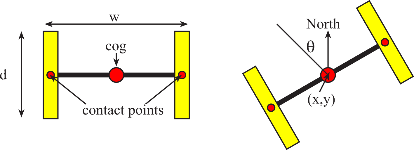
Figure 8.5.1. A robot with two drive wheels is defined by the wheelbase and wheel diameter.
Constants
Number of slots/rotation, n=32
Wheel diameter, d = 886 (0.01cm)


Figure 8.5.2. To measure wheel motion, we used an encoder on each wheel.
Wheelbase (distance between wheels), w = 1651 (0.01cm)
Wheel circumference, c = πd = 2783 (0.01cm)
Measurements
LCount the number of slots of left wheel in 349.5ms. RCount the number of slots of right wheel in 349.5ms. At 150 RPM, there will be 28 counts in 349.5 ms. Some simple cases are found in Table 8.5.1, where m is any number from ‑28 to +28.
|
LCount |
RCount |
Motion |
|
m |
m |
straight line motion in the current direction |
|
0 |
m |
pivot about stopped left motor |
|
m |
0 |
pivot about stopped right motor |
|
m |
-m |
pure rotation about cog |
Table 8.5.1. Example measurements, relationship between counts and motion.
Derivations
Lr = LCount *c/n the arc distance traveled by the left wheel (0.01cm)
Rr = RCount*c/n the arc distance traveled by the right wheel (0.01cm)
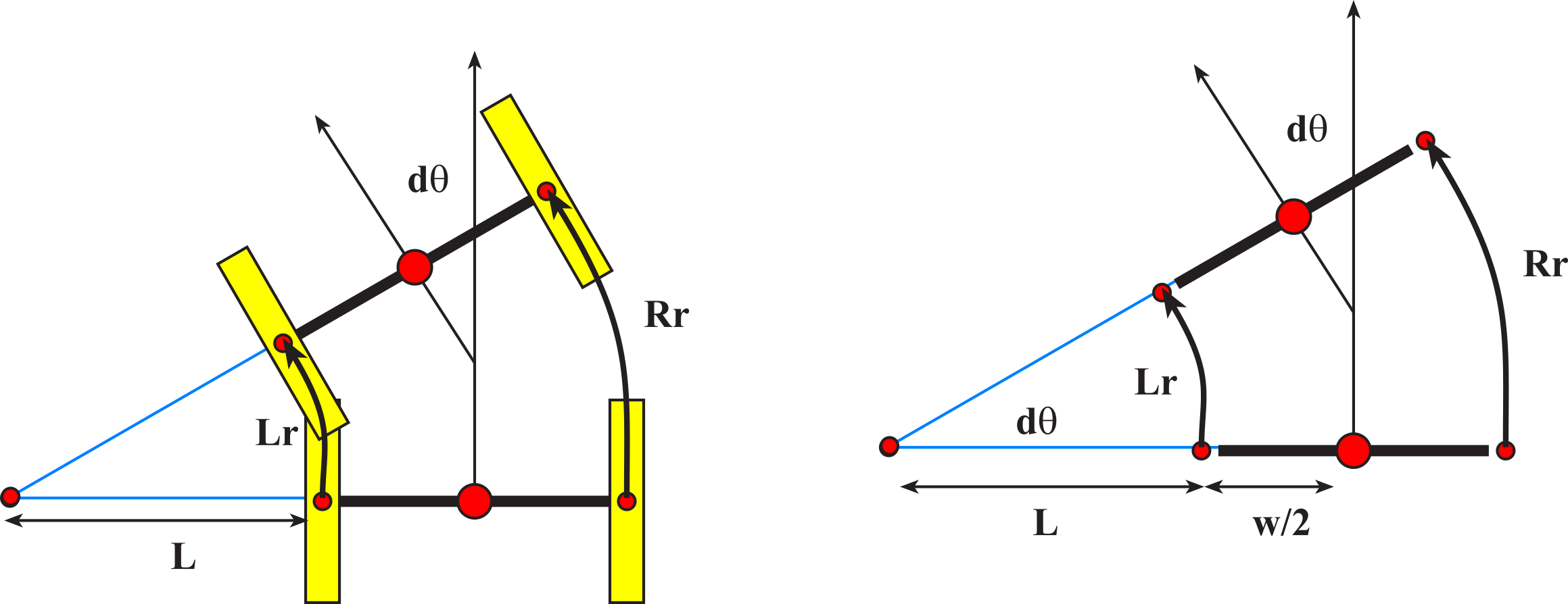
Figure 8.5.3. Motions occurring during a left turn.
Using similar triangles, we can find the new pivot point. Assuming Rr and Lr are both positive and Rr>Lr, we get
L/Lr = (L+w)/Rr
L/Lr - L/Rr = w/Rr
L Rr - L Lr = w Lr
L = w Lr/(Rr - Lr)
Notice also the change in yaw, dθ, is the same angle as the sector created by the change in axle. The change in angle is
dθ = Lr/L = Rr/(L+w)
We can divide the change in position into two components
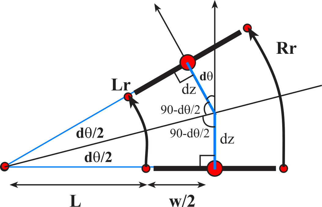
Figure 8.5.4. Geometry of a left turn.
The exact calculation for position change is
dz = (L+w/2)*tan(dθ/2)
but if dθ is small, we can approximate dz by the arc length.
dz = dθ/2*(L+w/2)
Initialize
We initialize the system by specifying the initial position and yaw.
(x, y, θ) (0.01cm, 0.01cm, 0.01 radian)
Calculations (run this periodically, measuring LCount RCount)
Lr = LCount *c/n (0.01cm)
Rr = RCount *c/n (0.01cm)
L = (w*Lr)/(Rr - Lr) (0.01cm)
dθ = (100*Lr)/L (0.01 radian)
dz = ((dθ/2)*(L+w/2))/100 (0.01cm) approximation
or dz = (tan(dθ/2)*(L+w/2))/100 (0.01cm) more accurate
x = x + dz*cos(θ) (0.01cm)
y = y+ dz*sin(θ) (0.01cm) first part of move
θ = θ + dθ (0.01 radian)
x = x + dz*cos(θ) (0.01cm)
y = y+ dz*sin(θ) (0.01cm) second part of move
A bang-bang controller uses a binary actuator, meaning the microcontroller output can be on or off. Other names for this controller are binary controller, two-position controller, and on/off controller. If there is a sensor that measures the status of the system, the controller can be closed loop. This signal is called the measurand or state variable. Assume when the actuator is on the measurand increases, and when the actuator is off, the measurand decreases. There is a desired point for the measurand. The bang-bang controller is simple. If the measurand is too small, the actuator is turned on, and if the measurand is too large the actuator is turned off. The controller sequence runs periodically:
1) Sample the sensor calculating the Measurand
2) If Measurand < Desired then TurnOn actuator else TurnOff actuator
This bang-bang controller can become unstable (actuator turns on and off repeatably when the Measurand equals Desired. We can remove the instability using hysteresis as described in the next example.
An example of a bang-bang controller is a heater that maintains the temperature as close to the desired temperature as possible (Figure 8.6.1). This is a closed-loop control system because the control signals (heat) depend on the state variables (temperature). In this application, the actuator has only two states: on that warms up the room and off that does not apply heat. For this application to function properly, there must be a passive heat loss that lowers the room temperature when the heater is turned off. On a hot summer day, this heater system will not be able to keep the house cool. A bang-bang controller turns on the power if the measured temperature is too low and turns off the power if the temperature is too high. To implement hysteresis, we need two set-point temperatures, Thigh and Tlow. The controller turns on the power (activate relay) if the temperature goes below Tlow and turns off the power (deactivate relay) if the temperature goes above Thigh. The difference Thigh - Tlow is called hysteresis. The hysteresis extends the life of the relay by reducing the number of times the relay opens and closes.

Figure 8.6.1. Flowchart of a Bang-Bang Temperature Controller.
Assume the function SE() returns the estimated temperature as a binary fixed-point number with a resolution of 0.5 °C. We can use a periodic interrupt so that the bang-bang controller runs in the background. The interrupt period is selected to be about the same as the time constant of the physical plant. The temperature variables Tlow, Thigh and T could be in any format, as long as the three formats are the same. The periodic interrupt performs these tasks
Calculate T = SE(); // units of 0.5 C
If T < Tlow, execute TurnOn(); // too cold, turn on heat
Else if T > Thigh, execute TurnOff(); // too hot, turn off heat
: What happens if Tlow and Thigh are too close together? What happens if Tlow and Thigh are too far apart?
Observation: Bang-bang control works well with a physical plant with a very slow response.
An incremental control system uses an actuator with a finite number of discrete output states. For example, the actuator might be a PWM output with 249 possibilities from 2, 3, 4, ... 249 (0 to 100%). It is a closed-loop control system, because there is a sensor that measures the state variable. Assume when the actuator increases the measurand increases, and when the actuator decreases, the measurand decreases. There is a desired point for the measurand. The incremental controller is simple. If the measurand is too small, the actuator is increased, and if the measurand is too large, the actuator is decreased. It is important to choose the rate to run the controller properly. A good rule of thumb is to run the controller about 10 times faster than the time constant of the plant. The control system should make sure the actuator signal remains in the appropriate range. E.g., you do not want to increment an actuator output of 255 and get 0! The incremental controller is usually slow, but it has good accuracy and is very stable.
The objective of this incremental control system is to control the speed, X, of a DC motor shown in Figure 8.6.2. We define X as the true speed, and X' as the measured speed, recognizing the state estimator might have errors. The actuator uses PWM to apply variable power, U, to the motor. A tachometer is used to measure speed, X'.
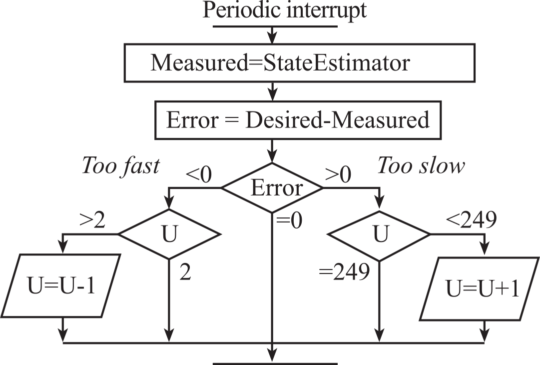
Figure 8.6.2. Flowchart of a position controller implemented using incremental control.
An incremental control algorithm simply adds or subtracts a constant from U depending on the sign of the error. In other words, if X' is too slow then U is incremented and if X' is too fast then U is decremented. It is important to choose the proper rate at which the incremental control software is executed. If it is executed too many times per second, then the actuator will saturate resulting in a Bang-Bang system. If it is not executed often enough then the system will not respond quickly to changes in the physical plant or changes in X*. In this incremental controller we add or subtract "1" from the actuator, but a value larger than "1" would have a faster response at the expense of introducing oscillations.
Common error: An error will occur if the software does not check for overflow and underflow after U is changed.
Observation: Many control systems operate well when the control equations are executed about 10 times faster than the step response time of the physical plant.
Assume the function SE() returns measured speed. We can use a periodic interrupt so that the incremental controller runs in the background. The interrupt period is selected to be about 10 times smaller than the time constant of the physical plant. The optimal controller rate depends on the significance of the ±1 value added to U. Experimental testing may be required to select an optimal controller rate, trading off response time for stability. Even though the position variables X' and Xstar may be unsigned, the error calculation E will be signed. Therefore, all controller variables will be defined as signed integers. Let K be a constant with the same units as X. The periodic interrupt performs these tasks
Measure X' = SE(); // estimated speed
E = Xstar - X'; // error
if E < -K then U--; // too fast, go slower
else if E > +K then U++; // too slow, go faster
if U < 2 then U=2; // underflow
else if U > 249 then U=249; // overflow
Update PWM_Duty(U);
: What happens if the interrupt period is too small (i.e., executes too frequently)?
Observation: It is a good debugging strategy to observe the assembly listing generated by the compiler when performing calculations on variables of mixed types (signed/unsigned, char/short).
Observation: Incremental control will work moderately well (accurate and stable) for an extremely wide range of applications. Its only shortcoming is that the controller response time can be quite slow.
8.7.1. General Approach to a PID Controller
The simple controllers presented in the last section are easy to implement but will have either large errors or very slow response times. To make a faster and more accurate system, we can use linear control theory to develop the digital controller. There are three components of a proportional integral derivative PID controller.

The error, E(t), is defined as the present set-point, X*(t), minus the measured value of the controlled variable, X'(t). See Figure 8.7.1.
E(t)=X*(t)- X'(t)
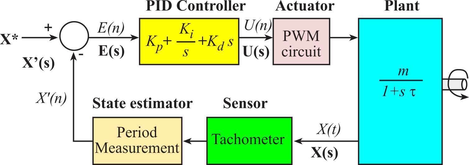
Figure 8.7.1. Block diagram of a linear control system in the frequency domain.
The PID controller calculates its output by summing three terms. The first term is proportional to the error. The second is proportional to the integral of the error over time, and the third is proportional to the rate of change (first derivative) of the error term. The values of Kp, Ki and Kd are design parameters and must be properly chosen in order for the control system to operate properly. The proportional term of the PID equation contributes an amount to the control output that is directly proportional to the current process error. The gain term Kp adjusts exactly how much the control output response should change in response to a given error level. The larger the value of Kp, the greater the system reaction to differences between the set-point and the actual state variable. However, if Kp is too large, the response may exhibit an undesirable degree of oscillation or even become unstable. On the other hand, if Kp is too small, the system will be slow or unresponsive. An inherent disadvantage of proportional-only control is its inability to eliminate the steady state errors (offsets) that occur after a set-point change or a sustained load disturbance.
The integral term converts the first order proportional controller into a second order system capable of tracking process disturbances. It adds to the controller output a factor that takes corrective action for any changes in the load level of the system. This integral term is scaled to the sum of all previous process errors in the system. As long as there is a process error, the integral term will add more amplitude to the controller output until the sum of all previous errors is zero. Theoretically, as long as the sign of Ki is correct, any value of Ki will eliminate offset errors. But, for extremely small values of Ki, the controlled variables will return to the set-point very slowly after a load upset or set-point change occurs. On the other hand, if Ki is too large, it tends to produce oscillatory response of the controlled process and reduces system stability. The undesirable effects of too much integral action can be avoided by proper tuning (adjusting) the controller or by including derivative action which tends to counteract the destabilizing effects.
The derivative action of a PID controller adds a term to the controller output scaled to the slope (rate of change) of the error term. The derivative term "anticipates" the error, providing a greater control response when the error term is changing in the wrong direction and a dampening response when the error term is changing in the correct direction. The derivative term tends to improve the dynamic response of the controlled variable by decreasing the process setting time, the time it takes the process to reach steady state. But if the process measurement is noisy, that is, if it contains high-frequency random fluctuations, then the derivative of the measured (controlled) variable will change wildly, and derivative action will amplify the noise unless the measurement is filtered.
: What happens in a PID controller if the sign of Ki is incorrect?
We can also use just some of the terms. For example, a proportional/integrator (PI) controller drops the derivative term. We will analyze the digital control system in the frequency domain. Let X(s) be the Laplace transform of the state variable x(t). Let X*(s) be the Laplace transform of the desired state variable x*(t). Let E(s) be the Laplace transform of the error
E(s) = X*(s) - X(s)
Let G(s) be the transfer equation of the PID linear controller. PID controllers are unique in this aspect. In other words, we cannot write a transfer equation for a bang-bang, incremental or fuzzy logic controller.

Let H(s) be the transfer equation of the physical plant. If we assume the physical plant (e.g., a DC motor) has a simple single pole behavior, then we can specify its response in the frequency domain with two parameters. m is the DC gain and t is its time constant. The transfer function of this simple motor is

The overall gain of the control system is

Theoretically we can choose controller constants, Kp Ki and Kd, to create the desired controller response. Unfortunately, it can be difficult to estimate m and t. If a load is applied to the motor, then m and t will change.
To simplify the PID controller implementation, we break the controller equation into separate proportion, integral and derivative terms. I.e., let
U(t) = P(t) + I(t) + D(t)
where U(t) is the actuator output, and P(t), I(t) and D(t) are the proportional, integral and derivative components respectively. The proportional term makes the actuator output linearly related to the error. Using a proportional term creates a control system that applies more energy to the plant when the error is large. To implement the proportional term, we simply convert it to discrete time.

where the index "n" refers to the discrete time input of E(n) and output of P(n).
Observation: To develop digital signal processing equations, it is imperative that the control system be executed on a regular and periodic rate.
Common error: If the sampling rate varies, then controller errors will occur.
The integral term makes the actuator output related to the integral of the error. Using an integral term often will improve the steady state error of the control system. If a small error accumulates for a long time, this term can get large. Some control systems put upper and lower bounds on this term, called anti-reset-windup, to prevent it from dominating the other terms. The implementation of the integral term requires the use of a discrete integral or sum. If I(n) is the current control output, and I(n-1) is the previous calculation, the integral term is simply

where ∆t is the sampling rate of E(n).
The derivative term makes the actuator output related to the derivative of the error. This term is usually combined with either the proportional and/or integral term to improve the transient response of the control system. The proper value of Kd will provide for a quick response to changes in either the set point or loads on the physical plant. An incorrect value may create an overdamped (very slow response) or an underdamped (unstable oscillations) response. There are a couple of ways to implement the discrete time derivative. The simple approach is

In practice, this first order equation is quite susceptible to noise. Figure 8.7.2 shows a sequence of E(n) with added noise. Notice that huge errors occur when the above equation is used to calculate the derivative.
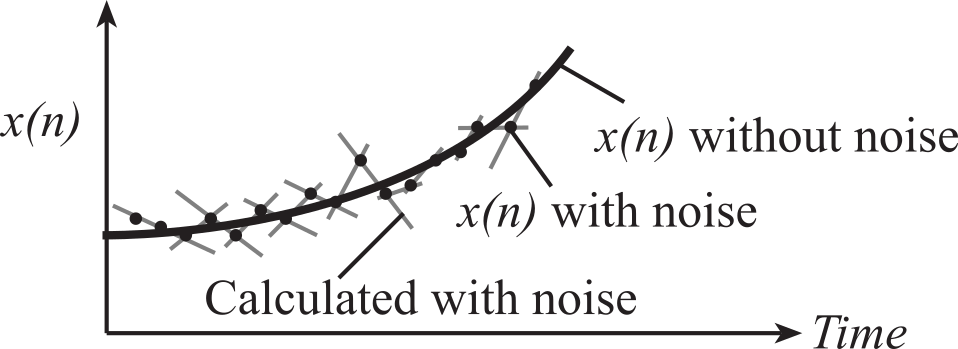
Figure 8.7.2. Illustration of the effect noise plays on the calculation of discrete derivative.
In most practical control systems, the derivative is calculated using the average of two derivatives calculated across different time spans. For example,

that simplifies to

Linear regression through multiple points can yield the slope and yet be immune to noise.
: How is the continuous integral related to the discrete integral?
: How is the continuous derivative related to the discrete derivative?
8.7.2. Design Process for a PID Controller
The first design step is the analysis phase, where we determine specifications such as range, accuracy, stability, and response time for our proposed control system. A data acquisition system will be used to estimate the state variables. Thus, its range, accuracy and response time must be better than the desired specifications of the control system. We can use time-based techniques using input capture or develop an ADC-based state estimator. In addition, we need to design an actuator to manipulate the state variables. It too must have a range and response time better than the controller specifications. The actuator resolution is defined as the smallest reliable change in output. For example, a 100 Hz PWM output generated by a 1 µsec clock has 10,000 different outputs. For this actuator, the actuator resolution is MaxPower/10000. We wish to relate the actuator performance to the overall objective of controller accuracy. Thus, we need to map the effect on the state variable caused a change in actuator output. This change in state variable should be less than or equal to the desired controller accuracy.
After the state estimator and actuator are implemented, the controller settings (KP, KI and KD) must be adjusted so that the system performance is satisfactory. This activity is referred to as controller tuning or field tuning. If you perform controller tuning by guessing the initial setting then adjusting them by trial and error, it can be tedious and time consuming. Thus, it is desirable to have good initial estimates of controller settings. A good first setting may be available from experience with similar control loops. Alternatively, initial estimates of controller settings can be derived from the transient response of the physical plant. A simple open-loop method, called the process reaction curve approach, was first proposed by Ziegler/Nichols and Cohen/Coon in 1953. In this discussion, the term "process" as defined by Ziegler/Nichols means the same thing as the "physical plant" described earlier in this chapter. This open-loop method requires only that a single step input be imposed on the process. The process reaction method is based on a single experimental test that is made with the controller in the manual mode. A small step change, ΔU, in the controller output is introduced and the measured process response is recorded, as shown in Figure 8.7.3. To obtain parameters of the process, a tangent is drawn to the process reaction curve at its point of maximum slope (at the inflection point). This slope is R, which is called the process reaction rate. The intersection of this tangent line with the original base line gives an indication of L, the process lag. L is really a measure of equivalent dead time for the process. If the tangent drawn at the inflection point is extrapolated to a vertical axis drawn at the time when the step was imposed, the amount by which this value is below the horizontal base line will be represented by the product L*R. ΔT is the time step for the digital controller. It is recommended to run P and PI controllers with ΔT = 0.1L, and a PID controller at a rate 20 times faster (ΔT = 0.05L.) Using these parameters, Ziegler and Nichol proposed initial controller settings as
Proportional Controller
Kp = ΔU/(L*R)
Proportional-Integral Controller
Kp = 0.9 ΔU/(L*R)
Ki = Kp /(3.33L)
Proportional-Integral-Derivative Controller
Kp = 1.2 ΔU/(L*R)
Ki = 0.5 Kp /L
Kd = 0.5 Kp L
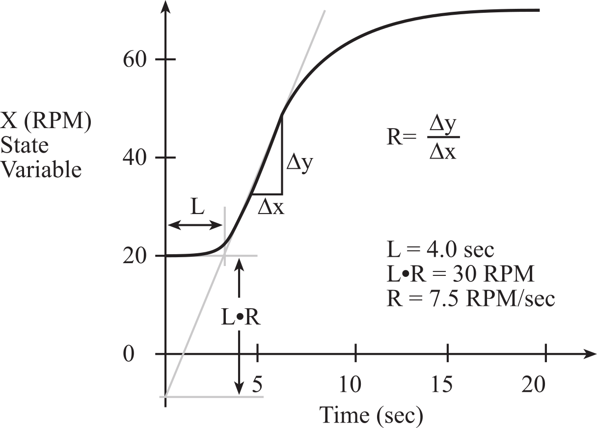
Figure 8.7.3. A process reaction curve used to determine controller settings.
: Are the Ziegler/Nichol equations consistent from a dimensional analysis perspective? In other words, are the units correct?
The response time is the delay after X* is changed for the system to reach a new constant state. Steady state controller accuracy is defined as the average difference between X* and X'. Overshoot is defined as the maximum positive error that occurs when X* is increased. Similarly, undershoot is defined as the maximum negative error that occurs when X* is decreased. During the testing phase, it is appropriate to add minimally intrusive debugging software that specifically measures performance parameters, such as response time, accuracy, overshoot, and undershoot. In addition, we can add instruments that allow us to observe the individual P(n), I(n) and D(n) components of the PID equation and their relation to controller error E(n).
Once the initial parameters are selected, a simple empirical method can be used to fine-tune the controller. This empirical approach starts with proportional term (Kp). As the proportional term is adjusted up or down, evaluate the quickness and smoothness of the controller response to changes in set-point and to changes in the load. Kp is too big if the actuator saturates both at the maximum and minimum after X* is changed. The next step is to adjust the integral term (Ki) a little at a time to improve the steady state controller accuracy without adversely affecting the response time. Don't change both Kp and Ki at once. Rather, you should vary them one at a time. If the response time, overshoot, undershoot and accuracy are within acceptable limits, then a PI controller is adequate. On the other hand, if accuracy and response are OK but overshoot and undershoot are unacceptable, adjust the derivative term (Kd) to reduce the overshoots and undershoots.
8.7.3. PI Controller Example
We will design a proportional-integral motor control system. The overall objective is to control the speed of an object with an accuracy of 0.1 RPM and a range of 0 to 100 RPM. Let X* be the desired state variable. In this example, X* will be a decimal fixed-point number and is set by the main program. Let X' be the estimated state variable that comes from the state estimator, which encodes the current position as the period of a squarewave, interfaced to an input capture pin. The period output of the sensor is linearly related to the speed X with a fixed offset. The accuracy of the state estimator needs to match the 0.1 RPM specification of the controller. If Delta is the measured period in bus cycles and X' is the estimated speed in 0.1 RPM, the state estimator measures the period and calculates X'. (see Section 8.2.4)
X' = 100133333333/Delta
Let U be the actuator control variable (100≤U≤19900). This system uses pulse width modulation with a 100 Hz squarewave that applies energy to the physical plant as shown in Figure 8.7.4. U will be the number of clock cycles (out of 20000) that the output is high. There is an external friction force slowing down on the motor. The PWM output from the computer creates a force causing the motor to spin faster.
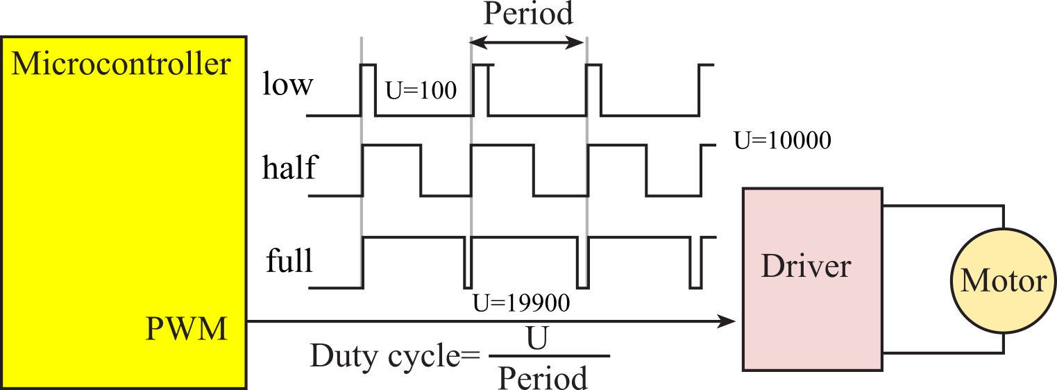
Figure 8.7.4. Pulse width modulated actuator signals.
The process reaction curve shown previously in Figure 8.7.3 was measured for this system after the actuator was changed from 250 to 2000, thus ΔU is 1750 (units of clock cycles). From Figure 8.7.3, the lag L is 4.0 sec and the process reaction rate R is 7.5RPM/sec. The controller rate is selected to be about 10 times faster than the lag L, so ΔT = 0.4 sec. In this way, the controller runs at a rate faster than the physical plant. We calculate the initial PI controller settings using the Ziegler/Nichol equations.
Kp = 0.9 ΔU/(L*R) = 0.9*1750/(4.0*7.5) = 52.5 cycles/RPM
Ki = Kp /(3.33L) = 52.5/(3.33*4.0) = 3.94144 cycles/RPM/sec
We will execute the PI control equation once every 0.4 second. X* and X' are decimal fixed-point numbers with a resolution of 0.1 RPM. The constant 52.5 is expressed as 105/2. The extra divide by 10 handles the decimal fixed-point representation of X* and X'. Notice 5.25 equals 336/64.
P(n) = Kp *(X*-X')/10 = 336*(X*-X')/64
We will also execute the integral control equation once every 0.4 second. Binary fixed-point is used to approximate 3.94144*0.4/10 as 2583/16384.
I(n) = I(n-1) + Ki •(X*-X')• ΔT/10
= I(n-1) + 3.94144 •(X*-X')•0.4/10 = I(n-1) + 101•(X*-X')/640
Program 8.7.1 shows an interrupt service handler, which runs every 0.4 second. Because the integral term will accumulate errors indefinitely, it is appropriate to put limits on the integral term. In this example, the integral term will remain between -500 and +19900. One must always limit the actuator output U to the physical limits of the PWM. The upper bound of the integral term will set the maximum actuator output. At steady state the proportional term will be 0, meaning the actuator output is set by the integral term.
int32_t X; // Estimated speed in 0.1 RPM, 0 to 1000
int32_t Xstar; // Desired speed in 0.1 RPM, 0 to 1000
int32_t E; // Speed error in 0.1 RPM, -1000 to +1000
int32_t U,I,P; // Actuator duty cycle, 100 to 19900 cycles
uint32_t Cnt; // incremented every 0.1 msec
int32_t Kp=336;
int32_t Ki=2583;
void Timer_Handler(void){ // runs every 0.4s
// 0<X<1000, 0<Xstar<1000, 100<U<19900
E = Xstar-X; // 0.1 RPM
P = (Kp*E)/64;
I = I+(Ki*E)/16364;
if(I < -500) I=-500; // anti-reset-windup
if(I > 19900) I=19900;
U = P+I; // PI controller has two parts
if(U < 100) U=100; // Constrain actuator output
if(U>19900) U=19900;
PWM_Duty(U); // output to actuator
// acknowledge periodic timer
}
Program 8.7.1. PI control software.
: What is the output U of the controller if the speed X is much greater than the set-point X*? In this situation, what does the object do?
Observation: PID control will work extremely well (fast, accurate and stable) if the physical plant can be described with a set of linear differential equations.
8.7.4. PID Controller Example
If the state estimator has very low noise, we can implement a PID controller. The derivative is calculated as the difference between this error and the previous error. The upper bound of the integral term will set the maximum actuator output. At steady state the proportional and derivative terms will be 0, meaning the actuator output is set by the integral term.
int32_t LastE,dEdt;
int32_t rps; // Estimated speed in rps
int32_t Xstar; // Desired speed in rps
int32_t E; // Speed error in rps
int32_t U,I,P,D // controller variables
uint32_t Cnt;
int32_t Kp;
int32_t Ki;
int32_t Kd;
void Timer_Handler(void){
Cnt++;
if(Cnt > 3){ // stopped motor
rps = 0; // set speed to zero
Cnt = 0;
}
E = Xstar-rps; // in rps
dEdt = E-LastE; // 0.1rpm/ms
P = (Kp * E)/1024; // Proportional term
if(P < -1000) P = -1000; // -1000 < P < +1000
if(P > 1000) P = 1000;
D = (Kd * dEdt)/1024; // Derivative term
if(D < -1000) D = -1000; // -1000 < D < +1000
if(D > 1000) D = 1000;
I = I + (Ki * E)/1024; // Integral term
if(I < -300) I = -1000; // -300 < I < 39900
if(I >39900) I = 39900;
U = P + I + D; // Calculate the actuator value
if(U < 300) U=300; // 300 < U < 39900
if(U >39900) U=39900;
PWM_Duty(U); // Send to PWM
LastE = E;
// acknowledge periodic timer
}
Program 8.7.2. PID control software.
: What error can be caused by running the controller too fast?
: What error can be caused by running the controller too slow?
In general, we adjust Ki to improve accuracy. In general, we adjust Kp to improve response time while minimizing ringing.
There are a number of reasons to consider fuzzy logic approach to control. It is much simpler than PI or PID systems. It will require less memory and execute faster. In other words, an 8-bit fuzzy system may perform as well (same steady state error and response time) as a 16-bit PID system. When complete knowledge about the physical plant is known, then a good PID controller can be developed. Since the fuzzy logic control is more robust (still works even if the parameter constants are not optimal), then the fuzzy logic approach can be used when complete knowledge about the plant is not known or can change dynamically. Choosing the proper PID parameters requires knowledge about the plant. The fuzzy logic approach is more intuitive, following more closely to the way a "human" would control the system. It is easy to modify an existing fuzzy control system into a new problem. The framework allows rapid prototyping.
Fuzzy logic was conceived in the mid-1960s by Lotfi Zadeh while at the University of California at Berkeley. However, the first commercial application didn't come until 1987, when the Matsushita Industrial Electric used it to control the temperature in a shower head. Named after the nineteenth-century mathematician George Boole, Boolean logic is an algebra where values are either true or false. This algebra includes operations of AND OR and NOT. Fuzzy logic is also an algebra, but where conditions may exist in the continuum between true and false. While Boolean logic defines two states, 8-bit fuzzy logic consists of 256 states all the way from "not at all" (0) to "definitely true" (255). "128" means half way between true and false. The fuzzy logic algebra also includes the operations of AND OR and NOT. A fuzzy membership set, a fuzzy variable, and a fuzzy set all refer to the same entity, which is a software variable describing the level of correctness for a condition within fuzzy logic. If we have a fuzzy membership set for the condition "hungry", then as the value of hungry moves from 0 to 255, the condition "hungry" becomes more and more true.
....0.....32.....64.....96.....128.....160.....192.....224.....255
Not at all ... a little bit ... somewhat ... mostly ... pretty much ... definitely
The design process for a fuzzy logic controller solves the following eight components. These components are listed in the order we would draw a data flow graph, starting with the state variables, progressing through the controller, and ending with the actuator output.
• The Physical plant has real state variables.
• The Data Acquisition System monitors these signals creating the estimated state variables.
• The Preprocessor may calculate relevant parameters called crisp inputs.
• Fuzzification will convert crisp inputs into input fuzzy membership sets.
• The Fuzzy Logic is a set of rules that calculate output fuzzy membership sets.
• Defuzzification will convert output sets into crisp outputs.
• The Postprocessor modify crisp outputs into a more convenient format.
• The Actuator System affects the Physical plant based on these outputs.
We will work through the concepts of fuzzy logic by considering examples of how we as humans control things like driving a car at a constant speed. During the initial stages of the design, we study the physical plant and decide which state variables to consider. For example, if we wish to control speed, then speed is obviously a state variable, but it might be also useful to know other forces acting on the object such as gravity (e.g., going up and down hills), wind speed and friction (e.g., rain and snow on the roadway). The purpose of the data acquisition system is to accurately measure the state variables. It is at this stage that the system converts physical signals into binary numbers to be processed by the software controller. We have seen two basic approaches in this book for this conversion: the measurement of period/frequency using input capture and the analog to digital conversion using an ADC. The preprocessor calculates crisp inputs, which are variables describing the input parameters in our software having units (like miles/hr). For example, if we measured speed, then some crisp inputs we might calculate would include speed error, and acceleration. Just like the PID controller, the accuracy of the data acquisition system must be better than the desired accuracy of the control system as a whole.
The next stage of the design is to consider the actuator and postprocessor. It is critical to be able to induce forces on the physical plant in a precise and fast manner. The step response of the actuator itself (time from software command to the application of force on the plant) must be faster than the step response of the plant (time from the application of force to the change in state variable.) Consider the case where we wish to control the temperature of a pot of water using a stove. The speed of the actuator is the time between turning the stove on and the time when heat is applied to the pot. The actuator on a gas stove is much faster than the actuator on an electric stove. The resolution of an actuator is the smallest change in output it can reliably generate. Just like the PID controller, the resolution of the actuator (converted into equivalent units on the input) must be smaller than the desired accuracy of the control system as a whole. A crisp output is a software variable describing the output parameters having units (like watts, Newtons, dynes/cm2 etc.). The postprocessor converts the crisp output into a form that can be directly output to the actuator. The postprocessor can verify the output signals are within the valid range of the actuator. One of the advantages of fuzzy logic design is the usage of human intuition. Think carefully about how you control the actuator (gas pedal) when attempting to drive a car at a constant speed. There is no parameter in your brain specifying the exact position of the pedal (e.g., 50% pressed, 65% pressed etc.), unless of course you are city taxicab driver (where your brain allows two actuator states: full gas and full brake.) Rather, what your brain creates as actuator commands are statements like "press the pedal little harder" and "press the pedal a lot softer." So, the crisp output of fuzzy logic controller might be change in pedal pressure ΔU, and the postprocessor would calculate U = U+ΔU, then check to make sure U is within an acceptable range.
We continue the design of a fuzzy logic controller by analyzing its crisp inputs. As a design step, we create a list of true/false conditions that together describe the current state of the physical plant. In particular, we define input fuzzy membership sets, which are fuzzy logic variables describing conditions related to the state of the physical plant. These fuzzy variables do not need to be orthogonal. In other words, it is acceptable to have variables that are related to each other. When designing a speed controller, we could define multiple fuzzy variables referring to similar conditions, such as WayTooFast, Fast, and LittleBitFast. Given the scenario where we are driving too fast, there should be generous overlap in conditions, such that two or even three fuzzy sets are simultaneously partially true. On the other hand, it is important that the entire list of input membership fuzzy sets, when considered as an ensemble, form a complete definition of the status of the physical plant. For example, if we are attempting to drive a car at a constant speed, then SlowingUp, GoingSteady, and SpeedingUp might be input fuzzy variables describing the car's acceleration. Fuzzification is the mathematical step converting the crisp inputs into input fuzzy membership sets. When implementing fuzzy logic explicitly with C code, we will have available the full set of AND, OR, NOT fuzzy logic operations.
The heart of a fuzzy logic controller is the fuzzy logic itself, which is set of logic equations that calculate fuzzy outputs as a function of fuzzy inputs. An output fuzzy membership set is a fuzzy logic variable describing a condition related to the actuator. QuickStop, SlowDown, JustRight, MorePower, and MaxPower are examples of output fuzzy variables that might be used to describe the action to perform on the gas pedal. Like input fuzzy variables, output fuzzy variables exist in the continuum from definitely false (0) to definitely true (1). Just like the input specification, it is also important to create a list of output membership fuzzy sets, when considered as an ensemble, form a complete characterization of what we wish to be able to do with the actuator. We write fuzzy logic equations using AND and OR functions in a way similar to Boolean logic. The fuzzy logic AND is calculated as the minimum value of the two inputs, and the fuzzy logic OR is calculated as the maximum value of the two inputs. The design of the rules, like the other aspects of fuzzy control, follows the human intuition.
SlowDown = WayTooFast + SpeedingUp*LittleBitFast
: If WayTooFast is 50, SpeedingUp is 40, and LittleBitFast is 60, then what would be the calculated value for SlowDown?
The defuzzification stage of the controller converts the output fuzzy variables into crisp outputs. Although any function could be used, an effective approach is to use a weighted average. Consider the case where the pedal pressure U varies from 0 to 100, thus the crisp output ΔU can take on values from -100 to +100. We think about what crisp output we want if just QuickStop were to be true. In this case, we wish to make ΔU equal to -100. We then define crisp output values for SlowDown, JustRight, MorePower, and MaxPower as -10, 0, +10, and +100 respectfully. We can combine the five factors using a weighted average.
![]()
Because the fuzzy controller is modular, we begin by testing each of the modules separately. The system-level testing of a fuzzy logic controller follows a procedure similar to the PID controller tuning. Debugging instruments can be added to record the crisp inputs, fuzzy inputs, fuzzy outputs, and crisp outputs during the real-time operation of the system. Fuzzification parameters are adjusted so that the status of the plant is captured in the set of values contained in the fuzzy input variables. Next, the rules are adjusted so that fuzzy output variables properly describe what we want to do with the actuator. Lastly, the defuzzification parameters are adjusted so the proper crisp outputs are created.
Next, we will design a fuzzy logic motor controller. The actuator is a PWM signal interfaced to the motor. The power to the motor is controlled by varying the 8-bit PWM duty cycle. The motor speed is estimated with a tachometer connected to an input capture pin.
Our system has:
• two control inputs
S* the desired motor speed in RPM
S' the current estimated motor speed RPM
• one control output
N the digital value that we write to the PWM
To utilize 8-bit math, we change the units of speed to 1000/256=3.90625 RPM.
T* =(256*S*)/1000 the desired motor speed in 3.9 RPM
T' =(256*S')/1000 the current estimated motor speed 3.9 RPM
For example, if the desired speed is 500 RPM, then T* will be 128. Notice that the estimated speed, T', is measured by the input capture pin. In other words, the control system functions (estimate state variables, control equation calculations, and actuator output) are performed on a regular and periodic basis, every ∆t time units. This allows signal processing techniques to the used. We will let T'(n) refer to the current measurement and T'(n-1) refer to the previous measurement, i.e., the one measured ∆t time ago.
In the fuzzy logic approach, we begin by considering how a "human" would control the motor. Assume your hand were on a joystick (or your foot on a gas pedal) and consider how you would adjust the joystick to maintain a constant speed. We select crisp inputs and outputs to base our control system on. It is logical to look at the error and the change in speed when developing a control system. Our fuzzy logic system will have two crisp inputs
E = T*-T' the error in motor speed in 3.9rpm
D = T'(n)-T'(n-1) the change in motor speed in 3.9rpm/time
Notice that if we perform the calculations of D on periodic intervals, then D will represent the derivative of T', dT'/dt. T* and T' are 8-bit unsigned numbers, so the potential range of E varies from -255 to +255. Errors beyond ±127 will be adjusted to the extremes +127 or -128 without loss of information.
int8_t static Subtract(uint8_t N, uint8_t M){
// returns N-M
uint32_t N16,M16;
int32_t Result16;
N16 = N; // Promote N,M
M16 = M;
Result16 = N16-M16; // -255≤Result16≤+255
if(Result16<-128) Result16 = -128;
if(Result16>127) Result16 = 127;
return(Result16);
}
Program 8.8.1. Subtraction with overflow/underflow checking.
These are the global definitions of the input signals and fuzzy logic crisp input,
uint8_t Ts; // Desired Speed in 3.9 rpm units
uint8_t T; // Current Speed in 3.9 rpm units
uint8_t Told; // Previous Speed in 3.9 rpm units
int8_t D; // Change in Speed in 3.9 rpm/time units
int8_t E; // Error in Speed in 3.9 rpm units
Program 8.8.2. Inputs and crisp inputs.
Common error: Neglecting overflow and underflow can cause significant errors.
The need for the special Subtract function can be demonstrated with the following example:
E = Ts-T; // if Ts=200 and T=50 then E will be -106!!
This function can be used to calculate both E and D,
void CrispInput(void){
E = Subtract(Ts,T);
D = Subtract(T,Told);
Told = T; // Set up Told for next time
}
Program 8.8.3. Calculation of crisp inputs.
Now, if Ts=200 and T=50 then E will be +127. To control the actuator, we could simply choose a new PWM value N as the crisp output. Instead, we will select, ∆N that is the change in N, rather than N itself because it better mimics how a "human" would control it. Again, think about how you control the speed of your car when driving. You do not adjust the gas pedal to a certain position, but rather make small or large changes to its position in order to speed up or slow down. Similarly, when controlling the temperature of the water in the shower, you do not set the hot/cold controls to certain absolute positions. Again you make differential changes to affect the "actuator" in this control system. Our fuzzy logic system will have one crisp output:
∆N change in output, N=N+∆N in PWM units
Next we introduce fuzzy membership sets that define the current state of the crisp inputs and outputs. Fuzzy membership sets are variables that have true/false values. The value of a fuzzy membership set ranges from definitely true (255) to definitely false (0). For example, if a fuzzy membership set has a value of 128, you are stating the condition is half way between true and false. For each membership set, it is important to assign a meaning or significance to it. The calculation of the input membership sets is called Fuzzification. For this simple fuzzy controller, we will define 6 membership sets for the crisp inputs:
Slow True if the motor is spinning too slow
OK True if the motor is spinning at the proper speed
Fast True if the motor is spinning too fast
Up True if the motor speed is getting larger
Constant True if the motor speed is remaining the same
Down True if the motor speed is getting smaller.
We will define 3 membership sets for the crisp output:
Decrease True if the motor speed should be decreased
Same True if the motor speed should remain the same
Increase True if the motor speed should be increased
The fuzzy membership sets are usually defined graphically, but software must be written to actually calculate each. In this implementation, we will define three adjustable thresholds, TE, TD and TN. These are software constants and provide some fine tuning to the control system. We will set each threshold to 20. If you build one of these fuzzy systems, try varying one threshold at a time and observe the system behavior (steady state controller error and transient response.) If the error, E, is -5 (3.9rpm units), the fuzzy logic will say that Fast is 64 (25% true), OK is 192 (75% true), and Slow is 0 (definitely false.) If the error, E, is +21 (in 3.9rpm units), the fuzzy logic will say that Fast is 0 (definitely false), OK is 0 (definitely false), and Slow is 255 (definitely true.) TE is defined to be the error (e.g., 20 in 3.9 rpm units is 78 rpm) above which we will definitely consider the speed to be too fast. Similarly, if the error is less than -TE, then the speed is definitely too slow.
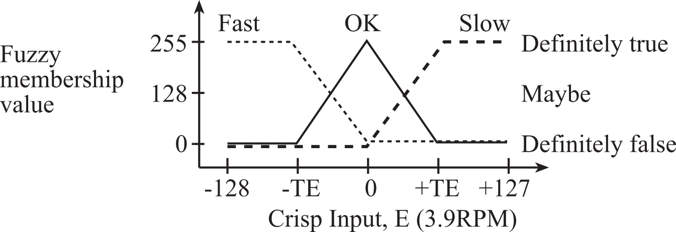
Figure 8.8.1. Fuzzification of the error input.
In this fuzzy system, the input membership sets are continuous piece-wise linear functions. Also, for each crisp input value, Fast, OK, Slow sum to 255. In general, it is possible for the fuzzy membership sets to be nonlinear or discontinuous, and the membership values do not have to sum to 255. The other three input fuzzy membership sets depend on the crisp input, D. TD is defined to be the change in speed (e.g., 20 in 3.9 rpm/time units is 78 rpm/time) above which we will definitely consider the speed to be going up. Similarly, if the change in speed is less than -TD, then the speed is definitely going down.
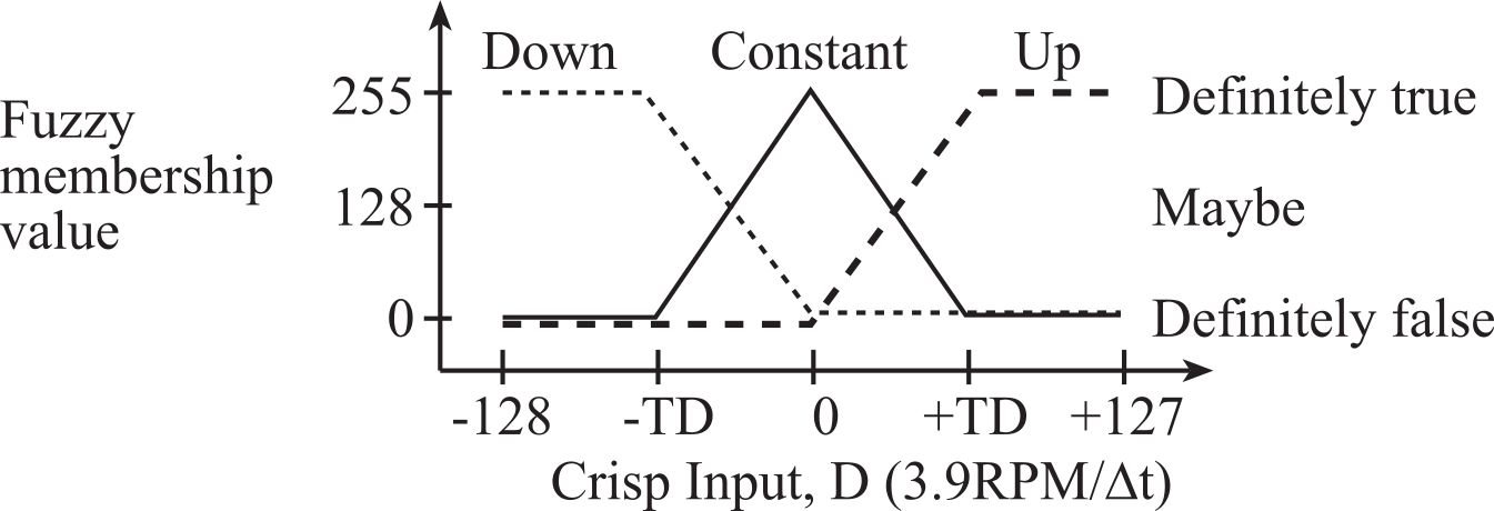
Figure 8.8.2. Fuzzification of the acceleration input.
In C, we could define a fuzzy function that takes the crisp inputs and calculates the fuzzy membership set values. Again, TE and TD are software constants that will affect the controller error and response time.
#define TE 20
uint8_t Fast, OK, Slow, Down, Constant, Up;
#define TD 20
uint8_t Increase,Same,Decrease;
#define TN 20
void InputMembership(void){
if(E <= -TE) { // E <= -TE
Fast = 255;
OK = 0;
Slow = 0;}
else
if(E < 0){ // -TE<E<0
Fast = (255*(-E))/TE;
OK = 255-Fast;
Slow = 0;}
else
if(E < TE){ // 0<E<TE
Fast = 0;
Slow = (255*E)/TE;
OK = 255-Slow;}
else { // +TE<=E
Fast = 0;
OK = 0;
Slow = 255;}
if(D <= -TD) { // D<=-TD
Down = 255;
Constant = 0;
Up = 0;}
else
if(D < 0){ // -TD<D<0
Down = (255*(-D))/TD;
Constant = 255-Down;
Up = 0;}
else
if(D < TD){ // 0<D<TD
Down = 0;
Up = (255*D)/TD;
Constant = 255-Up;}
else{ // +TD<=D
Down = 0;
Constant = 0;
Up = 255;
}
}
Program 8.8.4. Calculation of the fuzzy membership variables in C.
The fuzzy rules specify the relationship between the input fuzzy membership sets and the output fuzzy membership values. It is in these rules that one builds the intuition of the controller. For example, if the error is within reasonable limits and the speed is constant, then the output should not be changed. In fuzzy logic we write:
If OK and Constant then Same
If the error is within reasonable limits and the speed is going up, then the output should be reduced to compensate for the increase in speed. I.e.,
If OK and Up then Decrease
If the motor is spinning too fast and the speed is constant, then the output should be reduced to compensate for the error. I.e.,
If Fast and Constant then Decrease
If the motor is spinning too fast and the speed is going up, then the output should be reduced to compensate for both the error and the increase in speed. I.e.,
If Fast and Up then Decrease
If the error is within reasonable limits and the speed is going down, then the output should be increased to compensate for the drop in speed. I.e.,
If OK and Down then Increase
If the motor is spinning too slowly and the speed is constant, then the output should be increased to compensate for the error. I.e.,
If Slow and Constant then Increase
If the motor is spinning too slowly and the speed is going down, then the output should be increase to compensate for both the error and the drop in speed. I.e.,
If Slow and Down then Increase
These 7 rules can be illustrated in a table form.

Figure 8.8.3. Fuzzy logic rules shown in table form.
It is not necessary to provide a rule for all situations. For example, we did not specify what to do if Fast&Down or for Slow&Up. Although we could have added (but did not):
If Fast and Down then Same
If Slow and Up then Same
When more than one rule applied to an output membership set, then we can combine the rules:
Same=(OKandConstant)
Decrease=(OKandUp)or(FastandConstant)or(FastandUp)
Increase=(OKandDown)or(SlowandConstant)or(SlowandDown)
In fuzzy logic, the and operation is performed by taking the minimum and the or operation is the maximum. Thus the C function that calculates the three output fuzzy membership sets is
uint8_t static min(uint8_t u1,uint8_t u2){
if(u1>u2) return(u2);
else return(u1);
}
uint8_t static max(uint8_t u1,uint8_t u2){
if(u1<u2) return(u2);
else return(u1);
}
void OutputMembership(void){
Same = min(OK,Constant);
Decrease = min(OK,Up);
Decrease = max(Decrease,min(Fast,Constant));
Decrease = max(Decrease,min(Fast,Up));
Increase = min(OK,Down);
Increase = max(Increase,min(Slow,Constant));
Increase = max(Increase,min(Slow,Down));
}
Program 8.8.5. Calculation of the output fuzzy membership variables in C.
The calculation of the crisp outputs is called Defuzzification. The fuzzy membership sets for the output specifies the crisp output, ∆N, as a function of the membership value. For example, if the membership set Decrease were true (255) and the other two were false (0), then the change in output should be -TN (where TN is another software constant). If the membership set Same were true (255) and the other two were false (0), then the change in output should be 0. If the membership set Increase were true (255) and the other two were false (0), then the change in output should be +TN.
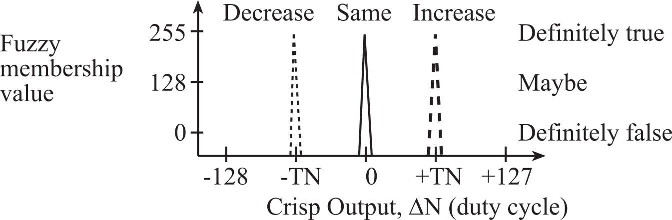
Figure 8.8.4. Defuzzification of the ∆N crisp output.
In general, we calculate the crisp output as the weighted average of the fuzzy membership sets:
∆N=(Decrease•(-TN) + Same•0 +Increase•TN)/(Decrease+Same+Increase)
The C compiler will promote the calculations to 32 bits and perform the calculation using 32-bit signed math that will eliminate overflow on intermediate terms. The output, dN, will be bounded in between -TN and +TN. Thus, the C function that calculates the crisp output is
int32_t dN,N;
void CrispOutput(void){
dN=(TN*(Increase-Decrease))/(Decrease+Same+Increase);
}
Program 8.8.6. Calculation of the crisp output in C.
void Timer_Handler(void){
T = SE(); // estimate speed, set T, 0 to 255
CrispInput(); // Calculate E,D and new Told
InputMembership(); // Sets Fast,OK,Slow,Down,Constant,Up
OutputMembership(); // Sets Increase,Same,Decrease
CrispOutput(); // Sets dN
N = max(0,min(N+dN,255));
PWM_Duty(N); // output to actuator, Section 2.8
// acknowledge timer periodic timer
}
Program 8.8.7. Periodic interrupt service for fuzzy logic controller.
Observation: Fuzzy logic control will work extremely well (fast, accurate and stable) if the designer has expert knowledge (intuition) of how the physical plant behaves.
8.9. RSLK Motor Controller Lab
Lab 8 for this course can be downloaded from this link Lab08.docx
Each lab also has a report Lab08Report.docx and
This work is based on the course ECE445L
taught at the University of Texas at Austin. This course was developed by Jonathan Valvano, Mark McDermott, and Bill Bard.
Reprinted with approval from Embedded Systems: Real-Time Interfacing to ARM Cortex-M Microcontrollers, ISBN-13: 978-1463590154

Embedded Systems: Real-Time Interfacing to ARM Cortex-M Microcontrollers by Jonathan Valvano is
licensed under a Creative
Commons
Attribution-NonCommercial-NoDerivatives 4.0 International License.