While you are preparing for the midterm, please keep in mind the course objectives:
Having regular sleep, eating, exercise and downtime from until the midterm exam will be very helpful in allowing you to have full mental energy for the test.
You can download a zip file of the files on the Canvas site prior to the midterm #1 exam.
Midterm #1 will be an in-person exam on Wednesday, March 11, 2026, from 10:30am to 11:45am, in one of two rooms:
The class average on midterm #1 has varied semester to semester. For the most recent in-person midterm #1 exams, the raw scores were 69.94 in fall 2021, 77.125 in spring 2022, 77.8 in spring 2023, and 73.2 in fall 2023.
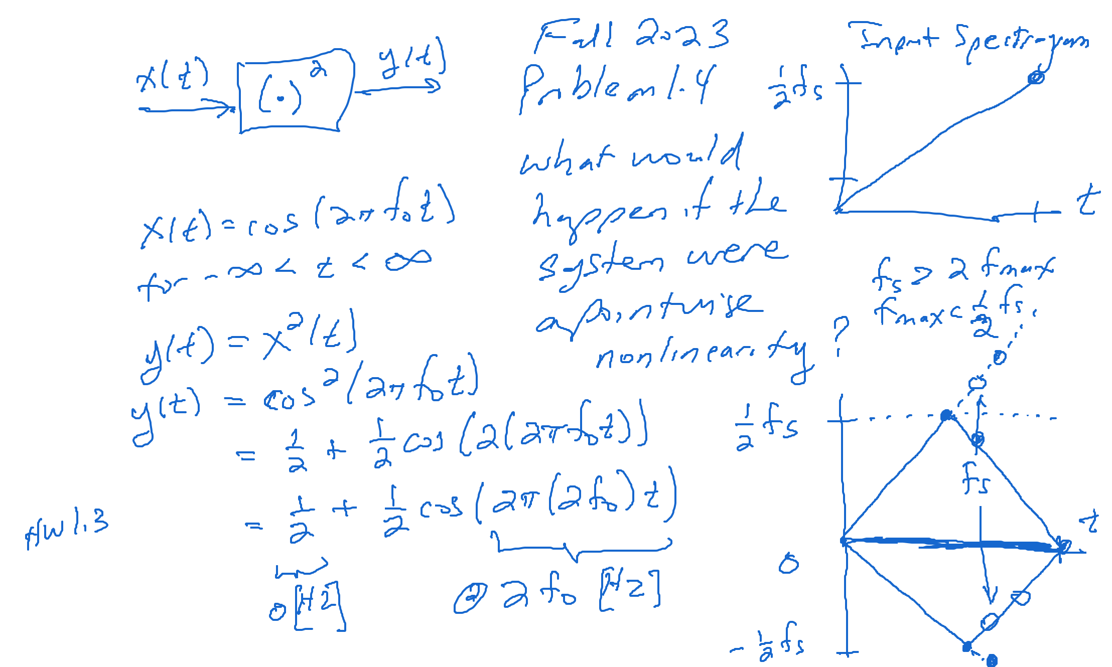
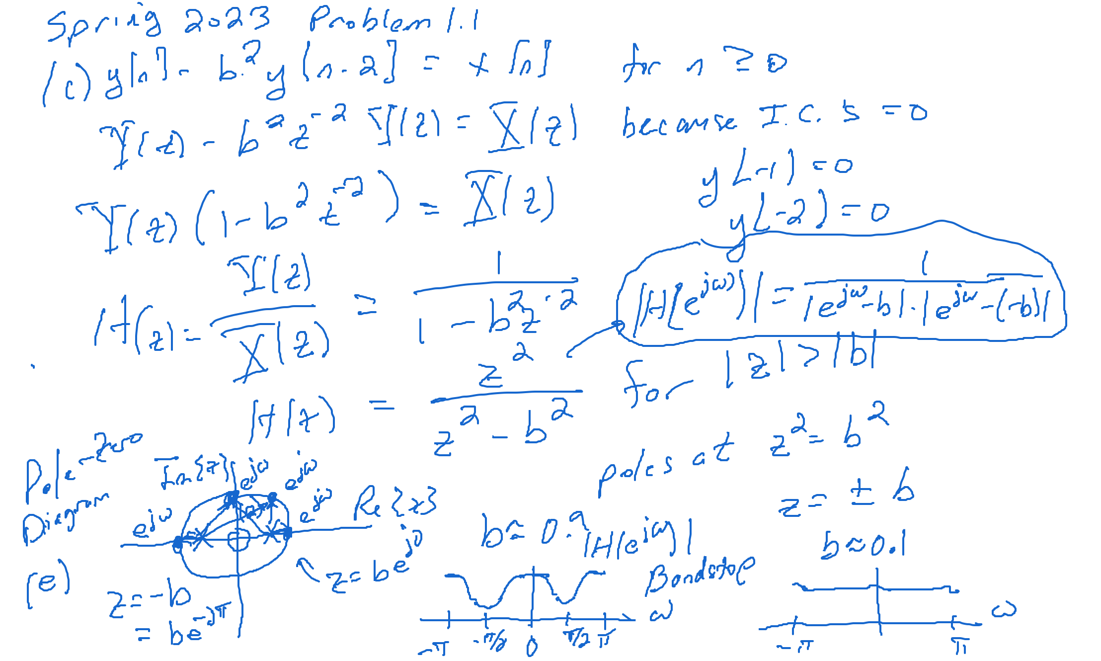
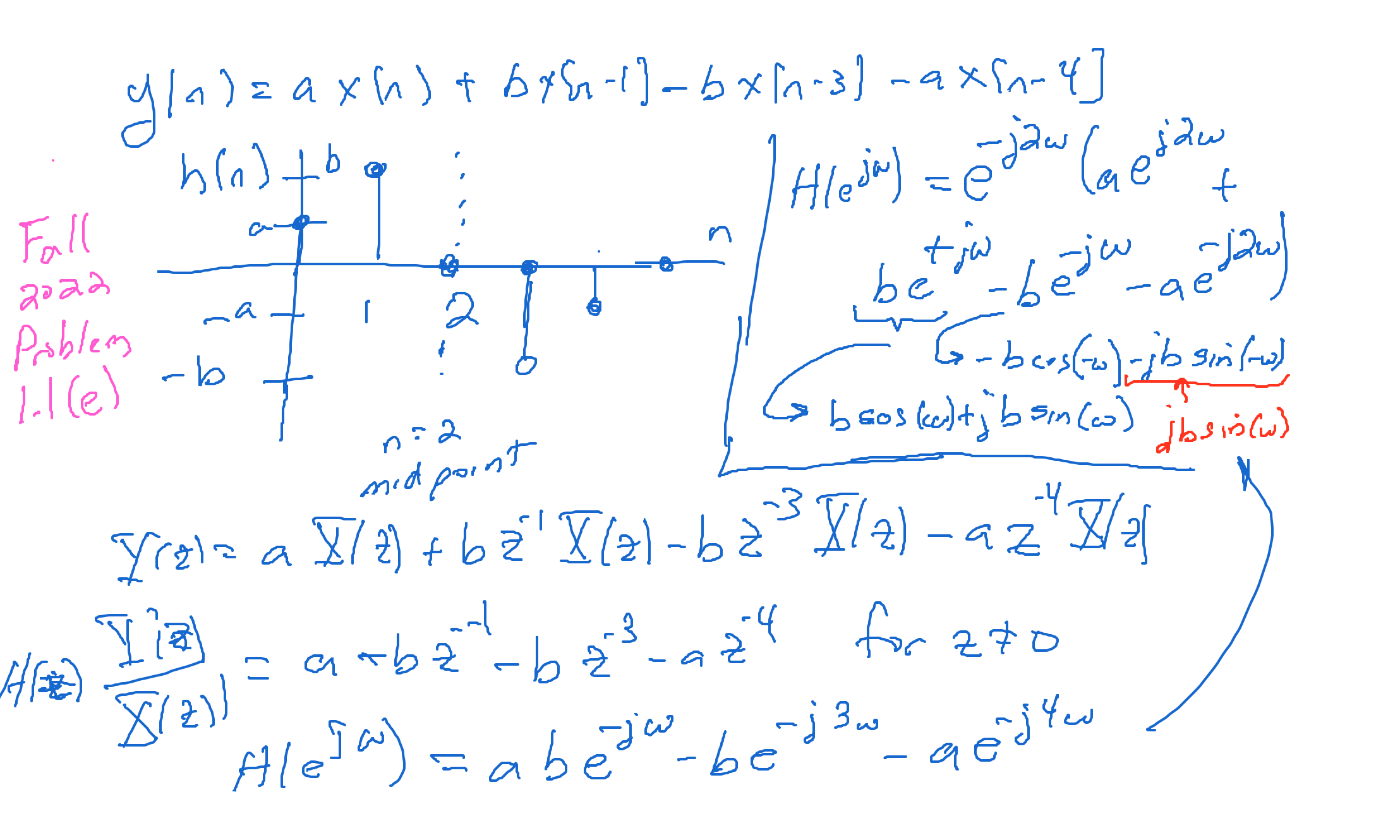
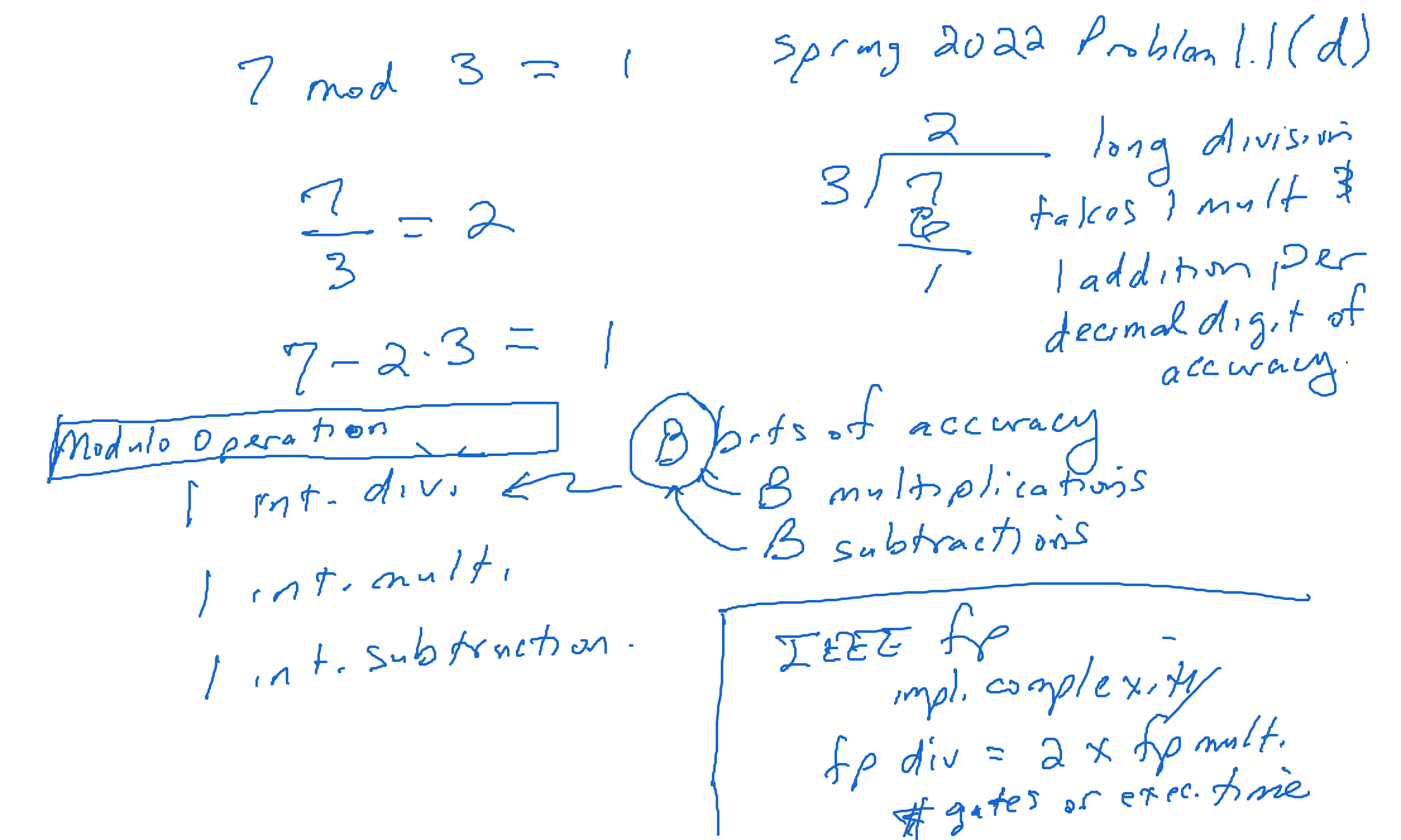
Here are several example midterm #1 exams:
Midterm #1 Review Slides are available from Spring 2017. The review slides are not comprehensive, but instead contain a sampling of important topics.
The online supplement to the book DSP First has dozens of worked problems from the pre-requisite course on signals and systems. After selecting a chapter on the Homework menu at the top right of the page, all of the problems from that chapter will be visible. There is a Solution button for those with solutions.
For Midterm #1, you will be responsible for the following topics in lectures 0-6, homework 0-3, labs 1-3, and the accompanying readings, handouts, and discussions. Below, JSK is Johnson, Sethares & Klein's Software Receiver Design. I've also included sections for three signals and systems textbooks as well: O&W is Oppenheim and Willsky's Signals and Systems (2nd ed.) SP First is McClellan, Schafer and Yoder's Signal Processing First, and L&G is Lathi and Green's Linear Systems and Signals (3rd ed.).
| Topic | Lectures | Lab | JSK | O&W | SP First | L&G | Homework Problems | Handouts |
| Introduction | 0 | 1 | Ch. 1 | |||||
| Bandwidth | 1 | 3 | Sec. 2.2 | Sec. 4.3-4.4 | Sec. 11-4 to 11-8 | Sec. 6.3-1, 7.2, 7.3, 7.9 | 0.1, 0.2, 1.2, 1.3, 2.2, 2.3, 3.1, 3.2, 3.3 | Introduction to Fourier Transforms and Pictorial dictionary of Fourier transforms (Canvas only) |
| Sinusoidal generation (oscillators) | 1 | 2 | Sec. 3.2 | 0.4 | ||||
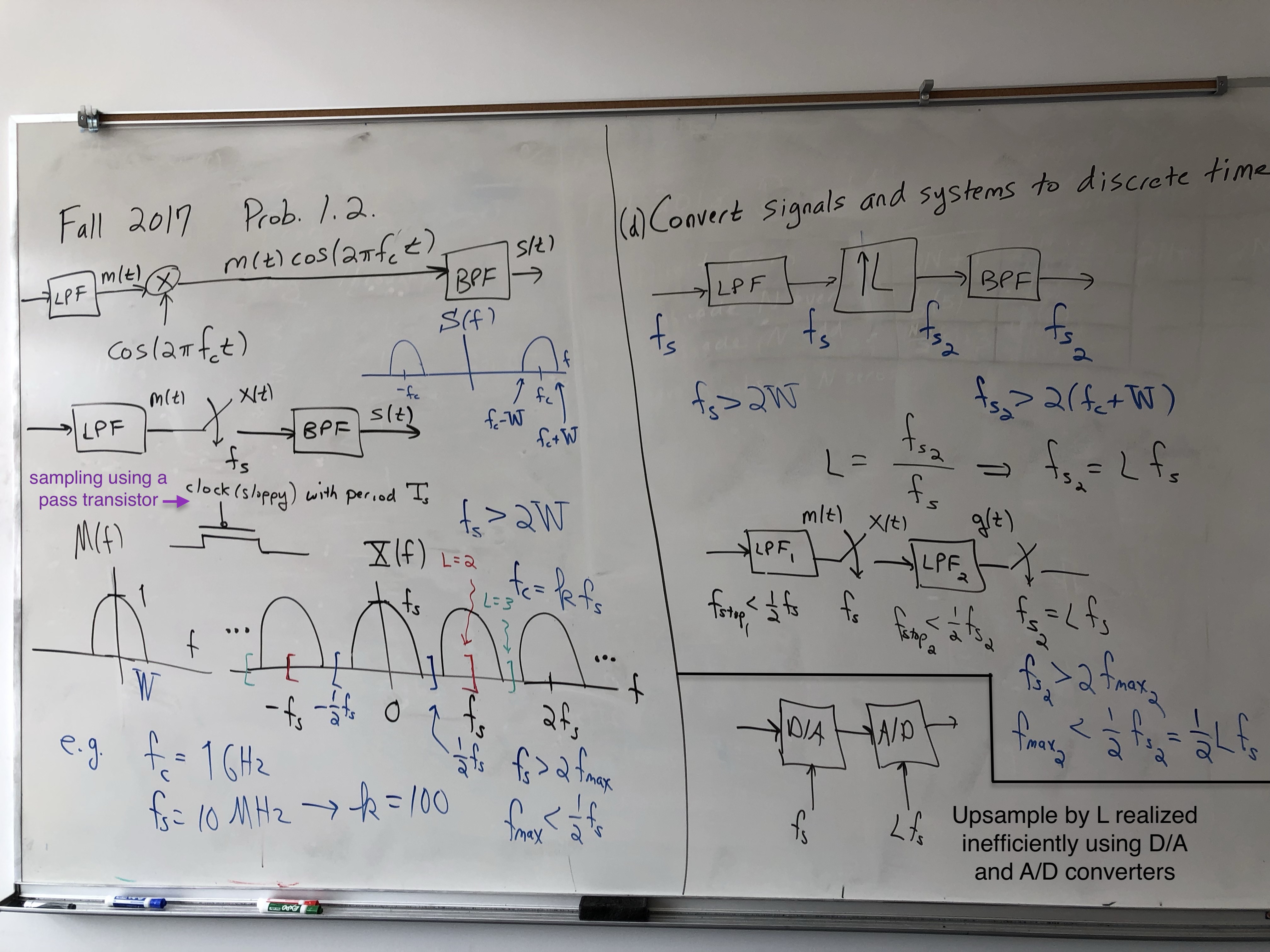
| Upconversion and downconversion | 1&4 | Sec. 2.3-2.6, 3.6; Ch. 5; Sec. 6.1-6.4 | Sec. 8.1-8.4 | Sec. 11-8.2 | Sec. 7.3, 7.7 | 0.1, 0.2, 0.3, 1.3, 3.2 | Sinusoidal Amplitude Modulation Example and Summary | |
| Communication system introduction | 1 | Ch. 1-2 | Ch. 8 | Sec. 7.7 | 0.2, 1.3, 3.2 | |||
| Basic continuous-time signals | 3 | 2 | Sec. 2.10, 4.3 | Sec. 1.3-1.4 | Sec. 2-3, 2-5, 4-4 & 9-1 | Sec. 1.4 | 0.1, 0.2, 0.3 | Common Signals in Matlab |
| Continuous-time system properties | 3 | Sec. 1.6 | Sec. 5-5 | Sec. 1.7 | 0.2, 1.3 | LTI System Properties, time invariance for an Ideal Delay and Integrator | ||
| Basic discrete-time signals | 3 | 1 | Sec. 1.3-1.4 | Sec. 4-2.1 & 5-3.2 | Sec. 3.3 | 0.1, 1.1, 1.2, 2.1 | Common Signals in Matlab; Discrete-Time Periodicity; and Chirp Signals | |
| Discrete-time system properties | 3 | 2&3 | Sec. 1.6 | Sec. 9-4 | Sec. 3.4-1 | 0.4, 1.1, 1.3, 2.1, 2.2, 2.3, 3.1, 3.2, 3.3 | LTI System Properties | |
| Fundamental Theorem of Linear Systems for continuous-time systems | 3&5 | Sec. 3.5 | Sec. 3.2 | Sec. 10-1 | Sec. 2.4-4 | 0.2 | Fundamental Theorem of Linear Systems | |
| Fundamental Theorem of Linear Systems for discrete-time systems | 3&5 | 3 | Sec. 3.5 | Sec. 3.2 | Sec. 6-1 | Sec. 3.8-2 | 1.1, 2.1, 2.2, 2.3, 3.1, 3.2, 3.3 | |
| Sampling theorem | 4 | 2 | Sec. 7.1 | Sec. 4-1, 4-2 & 4-5 | Sec. 8.1 | 0.1, 0.2, 0.3, 1.2, 1.3, 2.2, 3.2 | ||
| Sampling and aliasing | 4 | 2 | Sec. 2.8, 3.4, 6.1 | Sec. 7.3 an 7.4 | Sec. 12-3 | Sec. 8.2 | 0.1, 0.2, 0.3, 1.2, 1.3, 2.2, 3.2 | Sampling the Unit Step Function |
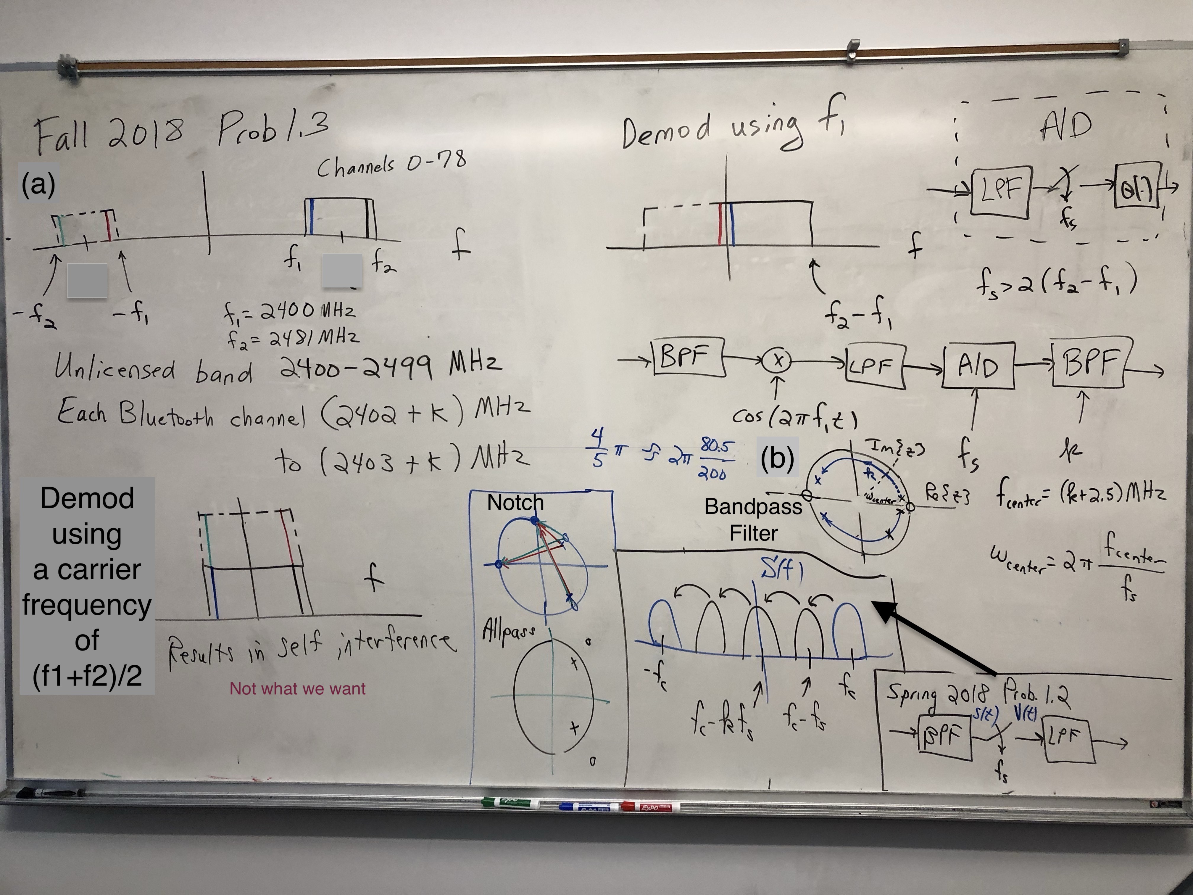
| Bandpass sampling | 4 | |||||||
| Discrete-time to continuous-time conversion | 4 | 2&3 | Sec. 2.10 & 6.4 | Sec. 7.2 | Sec. 4-4 | Sec. 8.2 | 1.2, 1.3, 2.2 (audio playback) | |
| Continuous-time convolution | 5 | Sec. 4.4 and 4.5 | Sec. 2.2 | Sec. 9-6 and 9-7 | Sec. 2.4 | Convolution Example | ||
| Discrete-time convolution | 5 | 3 | Sec. 4.4 and 4.5 | Sec. 2.1 | Sec. 5-3.3 and 5-6 | Sec. 3.8 | 1.3, 2.2, 3.1, 3.2 | Convolution Example and Four ways to filter a signal |
| Z-transforms | 5&6 | 3 | App. A.4 and F | Sec. 10.1-10.3, 10.5 | Sec. 7-1 to 7-5 | Sec. 5.1-5.2 | 0.4, 1.1 and 2.1 | |
| Transfer functions | 5&6 | 3 | Sec. 4.5 | Sec. 10.7.3, 10.7.4 and 10.8 | Sec. 8-3, 8-4 & 8-9 | Sec. 5.3 | 0.4, 1.1, 2.1 | Designing Averaging Filters and LTI Filters and Frequency Selectivity |
| Relationships between z and discrete-time Fourier transforms | 5 | 3 | App. F.2 | Sec. 10.4 | Sec. 7-6, 8-5, 8-6, and 8-10 | Sec. 5.5 | 1.1, 2.1, 2.3, 3.1, 3.3 | |
| Discrete-time FIR filter design & implementation | 5 | 3 | Sec. 2.12, 3.3, 4.2 | Sec. 10-9 | Sec. 7-7 | Sec. 5.4 | 1.3, 2.2, 3.1 | Four ways to filter a signal and Designing Averaging Filters |
| Digital FIR filter analysis | 5 | 3 | Ch. 7 and App. G | Sec. 7-7 to 7-9 | 1.1, 2.1 | Designing Averaging Filters | ||
| Stability of discrete-time LTI systems | 5&6 | 3 | Sec. 10.7.2 | Sec. 8-2.4, 8-4.2, and 8-8 | Sec. 3.9 and 3.10 | 1.1, 2.1, 3.3 | Bounded-Input Bounded-Output Stability | |
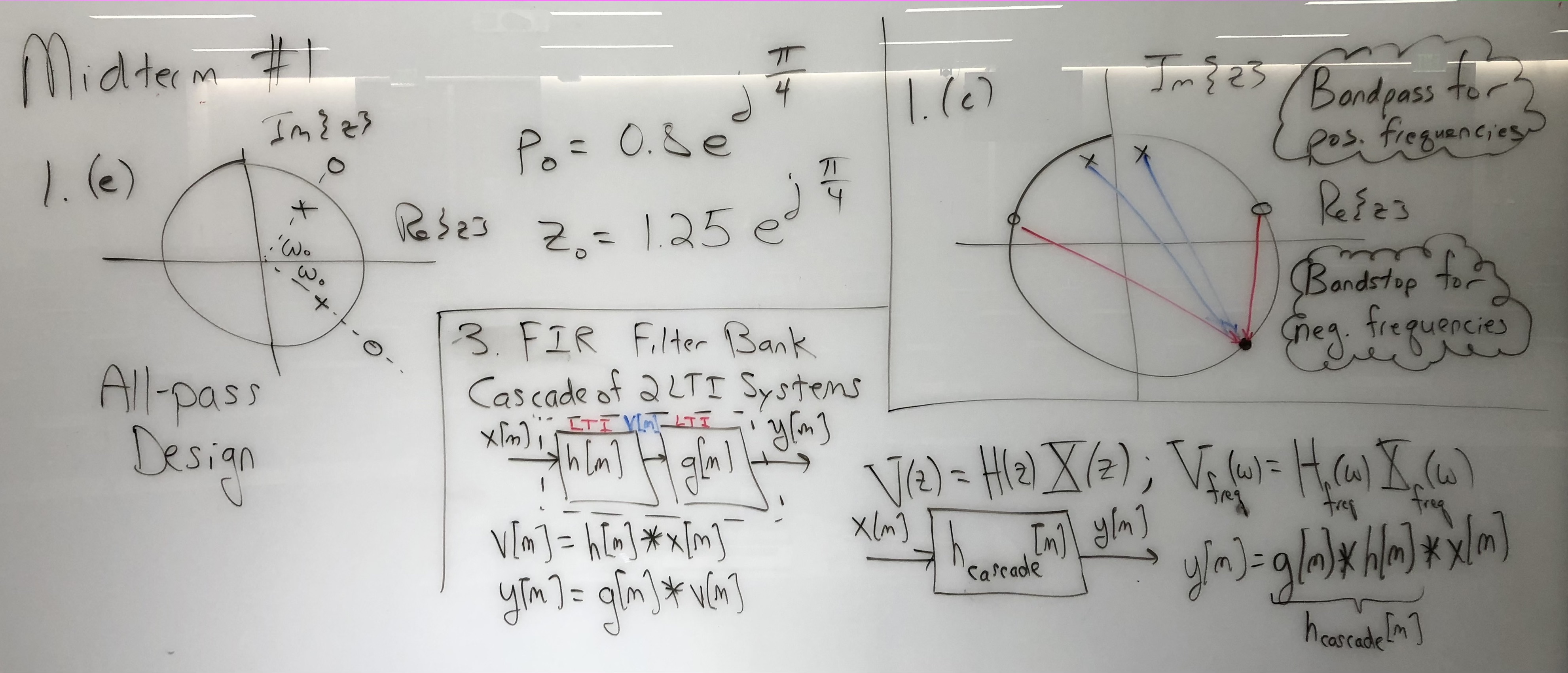
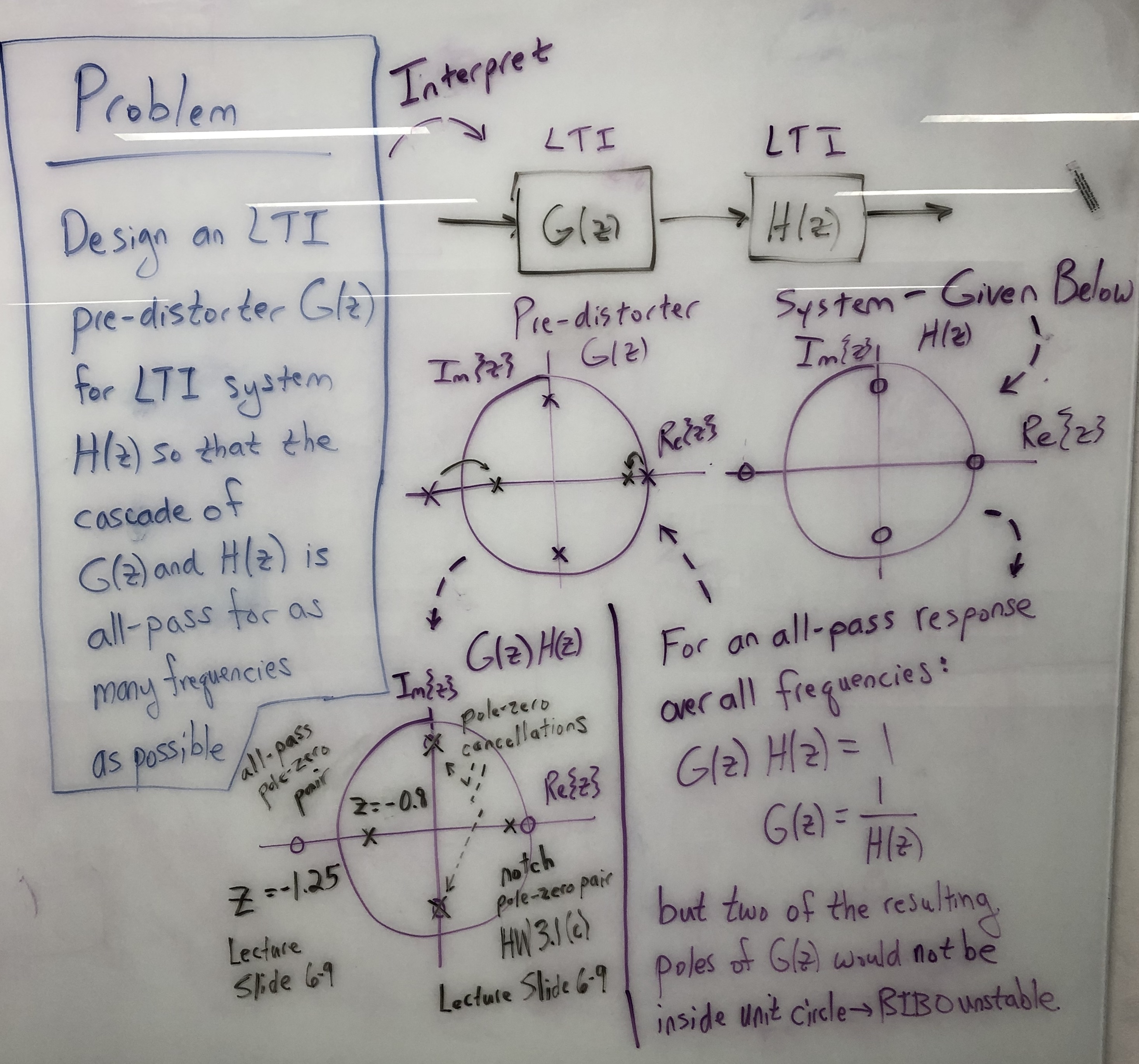
| Discrete-time IIR filter design by pole-zero placement | 6 | Sec. 10.4 | Sec. 8-9 and 8-10 | Sec. 5.6 | 1.1(d), 2.1(d), 3.1 | All-pass Filters | ||
| Classical discrete-time IIR filter design methods | 6 | 3 | Sec. 5.10 | 3.3 | Elliptic IIR filter design | |||
| Implementing discrete-time IIR filters as cascades of biquads | 6 | 3 | Sec. 10-9 | Sec. 8-9 | Sec. 5.4 | 3.3 | Parallel and Cascade Realizations of IIR Filters |
Please review the following demonstrations:
You won't be responsible for any questions specific to the assembly language, instruction set architecture, or C programming on the STM32h735G-DK ARM board. However, you would be responsible for analyzing run-time complexity of algorithms without any specific processor in mind. Run-time complexity includes memory storage, memory read/write rates, and buffered input/output. It will be important to know about common data types used in signal processing algorithms, such as 8-bit/16-bit/32-bit two's complement integers as well as IEEE 32-bit/64-bit floating-point data formats. These issues were covered in lab as well as homework questions 2.3 and 3.3 and lecture 6 on IIR filtering.
ii.png)
.png)